Note
Go to the end to download the full example code.
Band Structures of Bulk Structures#
Here, we calculate the band structure of relaxed bulk crystal structures.
Setting up bulk structures#
For more details regarding the set-up and relaxation of bulk structures, check out the Bulk Structures and Relaxations tutorial.
atoms = bulk('Ag')
Bulk DFT calculation#
For periodic DFT calculations we should generally use a number of
k-points which properly samples the Brillouin zone.
Many calculators including GPAW and Aims
accept the kpts keyword which can be a tuple such as
(4, 4, 4). In GPAW, the planewave mode
is very well suited for smaller periodic systems.
Using the planewave mode, we should also set a planewave cutoff (in eV):
Here we have used the setups keyword to specify that we want the
11-electron PAW dataset instead of the default which has 17 electrons,
making the calculation faster.
(In principle, we should be sure to converge both kpoint sampling and planewave cutoff – I.e., write a loop and try different samplings so we know both are good enough to accurately describe the quantity we want.)
Bulk Ag potential energy = -3.667eV
We can save the ground-state into a file
ground_state_file = 'bulk_Ag_groundstate.gpw'
calc.write(ground_state_file)
Density of states#
Having saved the ground-state, we can reload it for ASE to extract the density of states:
calc = GPAW(ground_state_file)
dos = DOS(calc, npts=800, width=0)
energies = dos.get_energies()
weights = dos.get_dos()
Calling the DOS class with width=0 means ASE calculates the DOS using
the linear tetrahedron interpolation method, which takes time but gives a
nicer representation. If the width is nonzero (e.g., 0.1 (eV)) ASE uses a
simple Gaussian smearing with that width, but we would need more k-points
to get a plot of the same quality.
fig, ax = plt.subplots()
ax.axvline(0.0, linestyle='--', color='black', alpha=0.5)
ax.plot(energies, weights)
ax.set_xlabel('Energy - Fermi Energy (eV)')
ax.set_ylabel('Density of States (1/eV)')
fig.tight_layout()
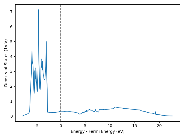
Time for analysis: Which parts of the spectrum do you think originate (mostly) from s electrons? And which parts (mostly) from d electrons?
As we probably know, the d-orbitals in a transition metal atom are localized close to the nucleus while the s-electron is much more delocalized.
In bulk systems, the s-states overlap a lot and therefore split into a very broad band over a wide energy range. d-states overlap much less and therefore also split less: They form a narrow band with a very high DOS. Very high indeed because there are 10 times as many d electrons as there are s electrons.
So to answer the question, the d-band accounts for most of the states forming the big, narrow chunk between -6.2 eV to -2.6 eV. Anything outside that interval is due to the much broader s band.
The DOS above the Fermi level may not be correct, since the SCF convergence criterion (in this calculation) only tracks the convergenece of occupied states. Hence, the energies over the Fermi level 0 are probably wrong.
What characterizes the noble metals Cu, Ag, and Au, is that the d-band is fully occupied. I.e.: The whole d-band lies below the Fermi level (energy=0). If we had calculated any other transition metal, the Fermi level would lie somewhere within the d-band.
Note
We could calculate the s, p, and d-projected DOS to see more conclusively which states have what character. In that case we should look up the GPAW documentation, or other calculator-specific documentation. So let’s not do that now.
Band structure#
Let’s calculate the band structure of silver.
First we need to set up a band path. Our favourite image search engine can show us some reference graphs. We might find band structures from both Exciting and GPAW with Brillouin-zone path:
\(\mathrm{W L \Gamma X W K}\).
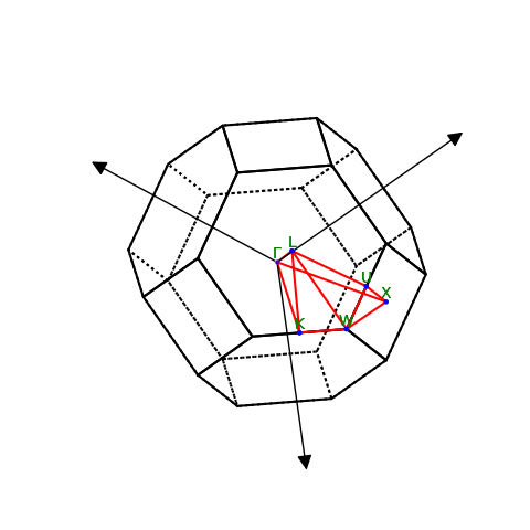
Luckily ASE knows these letters and can also help us visualize the reciprocal cell:
lat = atoms.cell.get_bravais_lattice()
print(lat.description())
FCC(a=4.09)
  Variant name: FCC
  Special point names: GKLUWX
  Default path: GXWKGLUWLK,UX

  Special point coordinates:
    G   0.0000  0.0000  0.0000
    K   0.3750  0.3750  0.7500
    L   0.5000  0.5000  0.5000
    U   0.6250  0.2500  0.6250
    W   0.5000  0.2500  0.7500
    X   0.5000  0.0000  0.5000
lat.plot_bz(show=True)
plt.show()
In general, the ase.lattice module provides
BravaisLattice classes used to represent each
of the 14 + 5 Bravais lattices in 3D and 2D, respectively.
These classes know about the high-symmetry k-points
and standard Brillouin-zone paths
(using the AFlow conventions).
You can visualize the band path object in bash via the command:
$ ase reciprocal path.json
You can print() the band path object to see some basic information
about it, or use its write() method
to save the band path to a json file such as path.json.
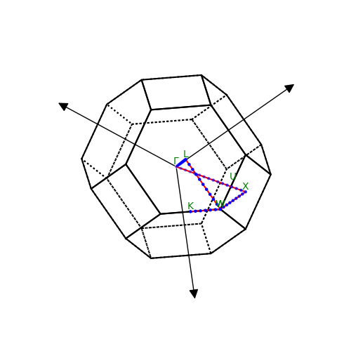
path = atoms.cell.bandpath('WLGXWK', density=10)
path.write('path.json')
print(path)
BandPath(path='WLGXWK', cell=[3x3], special_points={GKLUWX}, kpts=[53x3])
path.plot()
plt.show()
Once we are sure we have a good path with a reasonable number of k-points, we can run the band structure calculation. How to trigger a band structure calculation depends on which calculator we are using, so we would typically consult the documentation for that calculator (ASE will one day provide shortcuts to make this easier with common calculators):
calc = GPAW(ground_state_file)
calc = calc.fixed_density(kpts=path, symmetry='off')
  ___ ___ ___ _ _ _
 |   |   |_  | | | |
 | | | | | . | | | |
 |__ |  _|___|_____|  25.7.0
 |___|_|

User:   ???@runner-b6xc3srb6-project-71875181-concurrent-4
Date:   Mon May 25 16:01:12 2026
Arch:   x86_64
Pid:    1273
CWD:    /builds/ase/ase-deploy/examples/tutorials
Python: 3.13.7
gpaw:   /home/ase/.local/lib/python3.13/site-packages/gpaw
_gpaw:  /home/ase/.local/lib/python3.13/site-packages/
        _gpaw.cpython-313-x86_64-linux-gnu.so
ase:    /home/ase/.local/lib/python3.13/site-packages/ase (version 3.29.0b1)
numpy:  /home/ase/.local/lib/python3.13/site-packages/numpy (version 2.3.3)
scipy:  /home/ase/.local/lib/python3.13/site-packages/scipy (version 1.15.3)
libxc:  5.2.3
units:  Angstrom and eV
cores: 1
OpenMP: False
OMP_NUM_THREADS: 1

Input parameters:
  gpts: [14 14 14]
  kpts: {cell: Cell([[0.0, 2.0450000000000004, 2.0450000000000004], [2.0450000000000004, 0.0, 2.0450000000000004], [2.0450000000000004, 2.0450000000000004, 0.0]]),
         kpts: [[0.5        0.25       0.75      ]
 [0.5        0.275      0.725     ]
 [0.5        0.3        0.7       ]
 ...
 [0.41666667 0.33333333 0.75      ]
 [0.39583333 0.35416667 0.75      ]
 [0.375      0.375      0.75      ]],
         labelseq: WLGXWK,
         special_points: {'G': array([0., 0., 0.]), 'K': array([0.375, 0.375, 0.75 ]), 'L': array([0.5, 0.5, 0.5]), 'U': array([0.625, 0.25 , 0.625]), 'W': array([0.5 , 0.25, 0.75]), 'X': array([0.5, 0. , 0.5])}}
  mode: {ecut: 350.0,
         name: pw}
  setups: {Ag: 11}
  symmetry: off

Initialize ...

species:
  Ag:
    name: Silver
    id: aac732a7f42225a52edcbbb6e277d3cd
    Z: 47.0
    valence: 11
    core: 36
    charge: 0.0
    file: /home/ase/.local/lib/python3.13/site-packages/gpaw_data/setups/Ag.11.LDA.gz
    compensation charges: {type: gauss,
                           rc: 0.41,
                           lmax: 2}
    cutoffs: {filter: 2.31,
              core: 2.78}
    projectors:
      #              energy  rcut
      - 5s(1.00)    -4.708   1.296
      - 5p(0.00)    -0.844   1.296
      - 4d(10.00)    -7.664   1.296
      -  s          22.503   1.296
      -  p          26.368   1.296
      -  d          19.547   1.296

    # Using partial waves for Ag as LCAO basis

Reference energy: -144464.532254  # eV

Spin-paired calculation

Convergence criteria:
 Maximum [total energy] change in last 3 cyles: 0.0005 eV / valence electron
 Maximum integral of absolute [dens]ity change: 0.0001 electrons / valence electron
 Maximum integral of absolute [eigenst]ate change: 4e-08 eV^2 / valence electron
 Maximum number of scf [iter]ations: 333
 (Square brackets indicate name in SCF output, whereas a 'c' in
 the SCF output indicates the quantity has converged.)

Symmetries present (total): 1

  ( 1  0  0)
  ( 0  1  0)
  ( 0  0  1)

53 k-points
53 k-points in the irreducible part of the Brillouin zone
       k-points in crystal coordinates                weights
   0:     0.50000000    0.25000000    0.75000000       0.01886792
   1:     0.50000000    0.27500000    0.72500000       0.01886792
   2:     0.50000000    0.30000000    0.70000000       0.01886792
   3:     0.50000000    0.32500000    0.67500000       0.01886792
   4:     0.50000000    0.35000000    0.65000000       0.01886792
   5:     0.50000000    0.37500000    0.62500000       0.01886792
   6:     0.50000000    0.40000000    0.60000000       0.01886792
   7:     0.50000000    0.42500000    0.57500000       0.01886792
   8:     0.50000000    0.45000000    0.55000000       0.01886792
   9:     0.50000000    0.47500000    0.52500000       0.01886792
          ...
  52:     0.37500000    0.37500000    0.75000000       0.01886792

Wave functions: Plane wave expansion
  Cutoff energy: 350.000 eV
  Number of coefficients (min, max): 246, 271
  Pulay-stress correction: 0.000000 eV/Ang^3 (de/decut=0.000000)
  Using Numpy's FFT
  ScaLapack parameters: grid=1x1, blocksize=None
  Wavefunction extrapolation:
    Improved wavefunction reuse through dual PAW basis

Occupation numbers: Fermi-Dirac:
  width: 0.1000  # eV


Eigensolver
   Davidson(niter=2)

Densities:
  Coarse grid: 14*14*14 grid
  Fine grid: 28*28*28 grid
  Total Charge: 0.000000

Density mixing:
  Method: separate
  Backend: pulay
  Linear mixing parameter: 0.05
  old densities: 5
  Damping of long wavelength oscillations: 50

Hamiltonian:
  XC and Coulomb potentials evaluated on a 28*28*28 grid
  Using the LDA Exchange-Correlation functional
  External potential:
    NoExternalPotential


Memory estimate:
  Process memory now: 1349.92 MiB
  Calculator: 5.43 MiB
    Density: 1.02 MiB
      Arrays: 0.54 MiB
      Localized functions: 0.27 MiB
      Mixer: 0.21 MiB
    Hamiltonian: 0.36 MiB
      Arrays: 0.36 MiB
      XC: 0.00 MiB
      Poisson: 0.00 MiB
      vbar: 0.01 MiB
    Wavefunctions: 4.05 MiB
      Arrays psit_nG: 1.97 MiB
      Eigensolver: 0.07 MiB
      Projections: 0.13 MiB
      Projectors: 1.55 MiB
      PW-descriptor: 0.32 MiB

Total number of cores used: 1

Number of atoms: 1
Number of atomic orbitals: 9
Number of bands in calculation: 9
Number of valence electrons: 11
Bands to converge: occupied

... initialized

Initializing position-dependent things.

Creating initial wave functions:
  9 bands from LCAO basis set


       Ag


Atomic positions and initial magnetic moments

Positions:
   0 Ag     0.000000    0.000000    0.000000    ( 0.0000,  0.0000,  0.0000)

Unit cell:
           periodic     x           y           z      points  spacing
  1. axis:    yes    0.000000    2.045000    2.045000    14     0.1687
  2. axis:    yes    2.045000    0.000000    2.045000    14     0.1687
  3. axis:    yes    2.045000    2.045000    0.000000    14     0.1687

  Lengths:   2.892067   2.892067   2.892067
  Angles:   60.000000  60.000000  60.000000

Effective grid spacing dv^(1/3) = 0.1840

     iter     time        total  log10-change:
                         energy   eigst   dens
iter:   1 16:01:13    -4.699060               c
iter:   2 16:01:14    -4.702301   -1.99       c
iter:   3 16:01:14    -4.702813c  -2.74       c
iter:   4 16:01:15    -4.702925c  -3.38       c
iter:   5 16:01:15    -4.702951c  -4.02       c
iter:   6 16:01:16    -4.702957c  -4.64       c
iter:   7 16:01:16    -4.702958c  -5.25       c
iter:   8 16:01:16    -4.702958c  -5.86       c
iter:   9 16:01:17    -4.702959c  -6.43       c
iter:  10 16:01:17    -4.702959c  -6.98       c
iter:  11 16:01:18    -4.702959c  -7.52c      c

Converged after 11 iterations.

Dipole moment: (0.000000, -0.000000, -0.000000) |e|*Ang

Energy contributions relative to reference atoms: (reference = -144464.532254)

Kinetic:        -10.137585
Potential:       +7.854189
External:        +0.000000
XC:              -2.454638
Entropy (-ST):   -0.003366
Local:           +0.036759
SIC:             +0.000000
--------------------------
Free energy:     -4.704642
Extrapolated:    -4.702959

Showing only first 2 kpts
 Kpt  Band  Eigenvalues  Occupancy
  0     3      3.40599    2.00000
  0     4      4.40993    2.00000
  0     5     13.03013    0.00000
  0     6     13.03013    0.00000

  1     3      3.40507    2.00000
  1     4      4.37329    2.00000
  1     5     12.60044    0.00000
  1     6     12.65045    0.00000


Fermi level: 7.03906

No gap
No difference between direct/indirect transitions
We have here told GPAW to use our bandpath for k-points, not to perform symmetry-reduction of the k-points, and to fix the electron density.
Then we trigger a new calculation, which will be non-selfconsistent, and extract and save the band structure:
bs = calc.band_structure()
bs.write('bs.json')
print(bs)
BandStructure(path=BandPath(path='WLGXWK', cell=[3x3], special_points={GKLUWX}, kpts=[53x3]), energies=[1x53x9 values], reference=7.03906383347313)
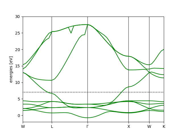
We can plot the band structure in python, or in the terminal from a file using:
$ ase band-structure bs.json
The plot will show the Fermi level as a dotted line (but does not define it as zero like the DOS plot before). Looking at the band structure, we see the complex tangle of what must be mostly d-states from before, as well as the few states with lower energy (at the \(\Gamma\) point) and higher energy (crossing the Fermi level) attributed to s.
ax = bs.plot()
ax.set_ylim(-2.0, 30.0)
plt.show()