Equation of state (EOS)

First, do a bulk calculation for different lattice constants:

import numpy as np

from ase import Atoms
from ase.calculators.emt import EMT
from ase.eos import EquationOfState
from ase.io import read
from ase.io.trajectory import Trajectory
from ase.units import kJ

a = 4.0  # approximate lattice constant
b = a / 2
ag = Atoms(
    'Ag', cell=[(0, b, b), (b, 0, b), (b, b, 0)], pbc=1, calculator=EMT()
)  # use EMT potential
cell = ag.get_cell()
traj = Trajectory('Ag.traj', 'w')
for x in np.linspace(0.95, 1.05, 5):
    ag.set_cell(cell * x, scale_atoms=True)
    ag.get_potential_energy()
    traj.write(ag)

This writes a trajectory file containing five configurations of FCC silver for five different lattice constants. Now, analyse the result with the EquationOfState class:

configs = read('Ag.traj@0:5')  # read 5 configurations
# Extract volumes and energies:
volumes = [ag.get_volume() for ag in configs]
energies = [ag.get_potential_energy() for ag in configs]
eos = EquationOfState(volumes, energies)
v0, e0, B = eos.fit()
print(B / kJ * 1.0e24, 'GPa')
eos.plot('Ag-eos.png')

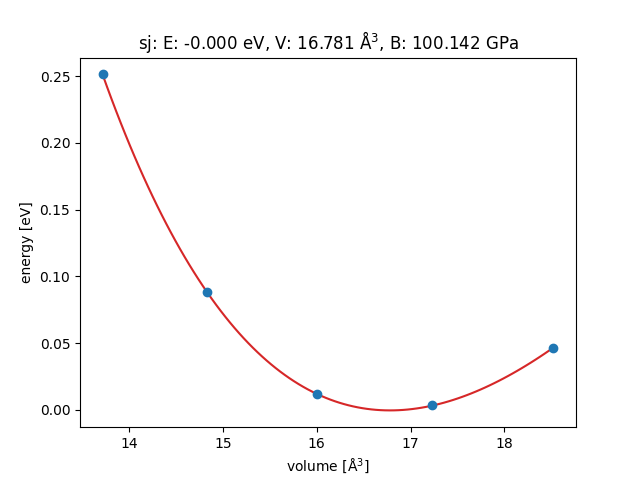
100.14189241973199 GPa

<Axes: title={'center': 'sj: E: -0.000 eV, V: 16.781 Å$^3$, B: 100.142 GPa'}, xlabel='volume [Å$^3$]', ylabel='energy [eV]'>

A quicker way to do this analysis is to use the ase.gui tool:

$   ase gui Ag.traj

And then choose Tools ‣ Bulk modulus.