ASE Introduction: Nitrogen on copper

This section gives a quick (and incomplete) overview of what ASE can do. You can download the code shown in this tutorial (and others in the same style) as python scripts or jupyter notebooks at the bottom of this page.

We will calculate the adsorption energy of a nitrogen molecule on a copper surface. This is done by calculating the total energy for the isolated slab and for the isolated molecule. The adsorbate is then added to the slab and relaxed, and the total energy for this composite system is calculated. The adsorption energy is obtained as the sum of the isolated energies minus the energy of the composite system.

You will be able to see an image of the system after relaxation, later in the “Visualization” section.

Please have a look at the following script:

from ase import Atoms
from ase.build import add_adsorbate, fcc111
from ase.calculators.emt import EMT
from ase.constraints import FixAtoms
from ase.optimize import QuasiNewton

h = 1.85
d = 1.10

slab = fcc111('Cu', size=(4, 4, 2), vacuum=10.0)

slab.calc = EMT()
e_slab = slab.get_potential_energy()

molecule = Atoms('2N', positions=[(0.0, 0.0, 0.0), (0.0, 0.0, d)])
molecule.calc = EMT()
e_N2 = molecule.get_potential_energy()

add_adsorbate(slab, molecule, h, 'ontop')
constraint = FixAtoms(mask=[a.symbol != 'N' for a in slab])
slab.set_constraint(constraint)
dyn = QuasiNewton(slab, trajectory='N2Cu.traj')
dyn.run(fmax=0.05)

print('Adsorption energy:', e_slab + e_N2 - slab.get_potential_energy())

                Step[ FC]     Time          Energy          fmax
BFGSLineSearch:    0[  0] 14:41:05       11.689927       1.0797
BFGSLineSearch:    1[  2] 14:41:05       11.670814       0.4090
BFGSLineSearch:    2[  4] 14:41:05       11.625880       0.0409
Adsorption energy: 0.3235194223176432

Assuming you have ASE setup correctly (Installation) you can copy it into a python file (e.g. N2Cu.py) and run the script:

python N2Cu.py

Please read below what the script does.

Atoms

The Atoms object is a collection of atoms. Here is how to define a N2 molecule by directly specifying the position of two nitrogen atoms

d = 1.10
molecule = Atoms('2N', positions=[(0.0, 0.0, 0.0), (0.0, 0.0, d)])

You can also build crystals using, for example, the lattice module which returns Atoms objects corresponding to common crystal structures. Let us make a Cu (111) surface

from ase.build import fcc111

slab = fcc111('Cu', size=(4, 4, 2), vacuum=10.0)

Adding calculator

In this overview we use the effective medium theory (EMT) calculator, as it is very fast and hence useful for getting started.

We can attach a calculator to the previously created Atoms objects

from ase.calculators.emt import EMT

slab.calc = EMT()
molecule.calc = EMT()

and use it to calculate the total energies for the systems by using the get_potential_energy() method from the Atoms class

e_slab = slab.get_potential_energy()
e_N2 = molecule.get_potential_energy()

Structure relaxation

Let’s use the QuasiNewton minimizer to optimize the structure of the N2 molecule adsorbed on the Cu surface. First add the adsorbate to the Cu slab, for example in the on-top position

h = 1.85
add_adsorbate(slab, molecule, h, 'ontop')

In order to speed up the relaxation, let us keep the Cu atoms fixed in the slab by using FixAtoms from the constraints module. Only the N2 molecule is then allowed to relax to the equilibrium structure

from ase.constraints import FixAtoms

constraint = FixAtoms(mask=[a.symbol != 'N' for a in slab])
slab.set_constraint(constraint)

Now attach the QuasiNewton minimizer to the system and save the trajectory file. Run the minimizer with the convergence criteria that the force on all atoms should be less than some fmax

from ase.optimize import QuasiNewton

dyn = QuasiNewton(slab, trajectory='N2Cu.traj')
dyn.run(fmax=0.05)

                Step[ FC]     Time          Energy          fmax
BFGSLineSearch:    0[  0] 14:41:05       11.689927       1.0797
BFGSLineSearch:    1[  2] 14:41:05       11.670814       0.4090
BFGSLineSearch:    2[  4] 14:41:05       11.625880       0.0409

np.True_

Note

The general documentation on structure optimizations contains information about different algorithms, saving the state of an optimizer and other functionality which should be considered when performing expensive relaxations.

Input-output

Writing the atomic positions to a file is done with the write() function

from ase.io import write

write('slab.xyz', slab)

/home/ase/.local/lib/python3.13/site-packages/ase/io/extxyz.py:318: UserWarning: Skipping unhashable information adsorbate_info
  warnings.warn('Skipping unhashable information '

This will write a file in the xyz-format. Possible formats are:

format	description
xyz	Simple xyz-format
cube	Gaussian cube file
pdb	Protein data bank file
traj	ASE’s own trajectory format
py	Python script

Reading from a file is done like this

from ase.io import read

slab_from_file = read('slab.xyz')

If the file contains several configurations, the default behavior of the write() function is to return the last configuration. However, we can load a specific configuration by doing

read('N2Cu.traj')  # last configuration
read('N2Cu.traj', -1)  # same as above
read('N2Cu.traj', 0)  # first configuration

Atoms(symbols='Cu32N2', pbc=[True, True, False], cell=[[10.210621920333747, 0.0, 0.0], [5.105310960166873, 8.842657971447272, 0.0], [0.0, 0.0, 22.08423447177455]], tags=..., constraint=FixAtoms(indices=[0, 1, 2, 3, 4, 5, 6, 7, 8, 9, 10, 11, 12, 13, 14, 15, 16, 17, 18, 19, 20, 21, 22, 23, 24, 25, 26, 27, 28, 29, 30, 31]), calculator=SinglePointCalculator(...))

Visualization

The simplest way to visualize the atoms is the view() function

from ase.visualize import view

view(slab)

<Popen: returncode: None args: ['/usr/local/bin/python3.13', '-m', 'ase', 'g...>

This will pop up a ase.gui window. Alternative viewers can be used by specifying the optional keyword viewer=... - use one of ‘ase.gui’, ‘gopenmol’, ‘vmd’, or ‘rasmol’. (Note that these alternative viewers are not a part of ASE and will need to be installed by the user separately.) The VMD viewer can take an optional data argument to show 3D data

view(slab, viewer='VMD', data=array)

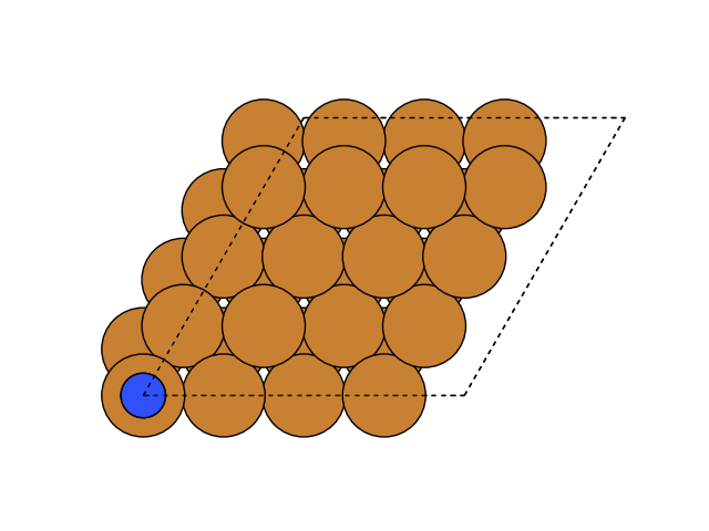
If you do not want a gui to open and plot this directly, you can do this with plot_atoms in Matplotlib

import matplotlib.pyplot as plt

from ase.visualize.plot import plot_atoms

fig, ax = plt.subplots()
plot_atoms(slab_from_file, ax)
ax.set_axis_off()

Molecular dynamics

Let us look at the nitrogen molecule as an example of molecular dynamics with the VelocityVerlet algorithm. We first create the VelocityVerlet object giving it the molecule and the time step for the integration of Newton’s law. We then perform the dynamics by calling its run() method and giving it the number of steps to take:

from ase import units
from ase.md.verlet import VelocityVerlet

dyn = VelocityVerlet(molecule, timestep=1.0 * units.fs)
for i in range(10):
    pot = molecule.get_potential_energy()
    kin = molecule.get_kinetic_energy()
    print('%2d: %.5f eV, %.5f eV, %.5f eV' % (i, pot + kin, pot, kin))
    dyn.run(steps=20)

0: 0.44034 eV, 0.44034 eV, 0.00000 eV
1: 0.43816 eV, 0.26289 eV, 0.17527 eV
2: 0.44058 eV, 0.43142 eV, 0.00916 eV
3: 0.43874 eV, 0.29292 eV, 0.14582 eV
4: 0.44015 eV, 0.41839 eV, 0.02176 eV
5: 0.43831 eV, 0.28902 eV, 0.14929 eV
6: 0.43947 eV, 0.36902 eV, 0.07045 eV
7: 0.43951 eV, 0.35507 eV, 0.08444 eV
8: 0.43959 eV, 0.36221 eV, 0.07738 eV
9: 0.43933 eV, 0.36044 eV, 0.07889 eV