
Equation of state (EOS)#
Note
We are currently moving to a new way to display our examples. For this example we have an updated version, which you can find here. The example on this page is deprecated and will be removed once all examples have been moved to the new format.
First, do a bulk calculation for different lattice constants:
import numpy as np

from ase import Atoms
from ase.calculators.emt import EMT
from ase.io.trajectory import Trajectory

a = 4.0  # approximate lattice constant
b = a / 2
ag = Atoms(
    'Ag', cell=[(0, b, b), (b, 0, b), (b, b, 0)], pbc=1, calculator=EMT()
)  # use EMT potential
cell = ag.get_cell()
traj = Trajectory('Ag.traj', 'w')
for x in np.linspace(0.95, 1.05, 5):
    ag.set_cell(cell * x, scale_atoms=True)
    ag.get_potential_energy()
    traj.write(ag)
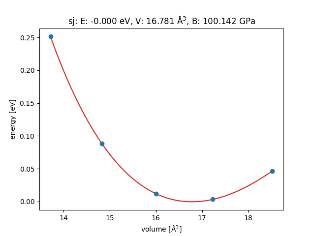
This will write a trajectory file containing five configurations of
FCC silver for five different lattice constants. Now, analyse the
result with the EquationOfState class and this
script:
from ase.eos import EquationOfState
from ase.io import read
from ase.units import kJ

configs = read('Ag.traj@0:5')  # read 5 configurations
# Extract volumes and energies:
volumes = [ag.get_volume() for ag in configs]
energies = [ag.get_potential_energy() for ag in configs]
eos = EquationOfState(volumes, energies)
v0, e0, B = eos.fit()
print(B / kJ * 1.0e24, 'GPa')
eos.plot('Ag-eos.png')
A quicker way to do this analysis, is to use the ase.gui tool:
$ ase gui Ag.traj
And then choose .