Structure optimization: H₂O

Let’s calculate the structure of the H₂O molecule. Part of this tutorial is exercise-based, so refer back to what you learnt from ASE Introduction: Nitrogen on copper and Atoms and calculators. Suggested solutions to the exercises are found after each exercise, but try solving them youself first!

Exercise

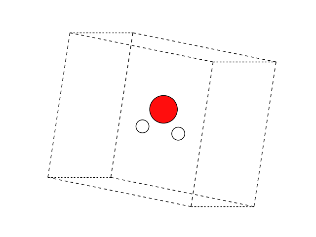
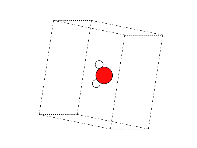
Create an Atoms object representing an H₂O molecule by providing chemical symbols and a guess for the positions. Visualize it, making sure the molecule is V shaped.

Solution:

import matplotlib.pyplot as plt

from ase import Atoms
from ase.visualize.plot import plot_atoms

atoms = Atoms('HOH', positions=[[0, 0, -1], [0, 1, 0], [0, 0, 1]])
atoms.center(vacuum=3.0)

fig, ax = plt.subplots()
plot_atoms(atoms, ax, rotation='10x,60y,0z')
ax.set_axis_off()

Exercise

Run a self-consistent calculation of the approximate H₂O molecule using GPAW.

Solution:

from gpaw import GPAW

calc = GPAW(mode='lcao', basis='dzp', txt='gpaw.txt')
atoms.calc = calc

Optimizers

We will next want to optimize the geometry. ASE provides several optimization algorithms that can run on top of Atoms equipped with a calculator:

Exercise

Run a structure optimization, thus calculating the equilibrium geometry of H₂O.

Solution:

from ase.optimize import BFGS

opt = BFGS(atoms, trajectory='opt.traj', logfile='opt.log')
opt.run(fmax=0.05)

np.True_

The trajectory keyword above ensures that the trajectory of intermediate geometries is written to opt.traj.

Exercise

Visualize the output trajectory and play it as an animation. Use the mouse to drag a box around and select the three atoms — this will display the angles between them. What is H–O–H angle of H₂O?

Solution:

from ase.io import read
from ase.visualize import view

atoms = read('opt.traj', ':')
view(atoms)

Note that the above will open in a separate graphical window. As always in ASE, we can do things programmatically, too, if we know the right incantations:

from ase.io import read

atoms = read('opt.traj', ':')
print(atoms[-1].get_angle(0, 1, 2))
print(atoms[-1].get_angle(2, 0, 1))
print(atoms[-1].get_angle(1, 2, 0))

103.45874999691222
38.27062500154389
38.270625001543884

The documentation on the Atoms object provides a long list of methods.

G2 molecule dataset

ASE knows many common molecules, so we did not really need to type in all the molecular coordinates ourselves. As luck would have it, the ase.build.molecule() function does exactly what we need:

from ase.build import molecule

atoms = molecule('H2O', vacuum=3.0)
fig, ax = plt.subplots()
plot_atoms(atoms, ax, rotation='10x,60y,0z')
ax.set_axis_off()

This function returns a molecule from the G2 test set, which is nice if we remember the exact name of that molecule, in this case ‘H₂O’. In case we don’t have all the molecule names memorized, we can work with the G2 test set using the more general ase.collections.g2 module:

from ase.collections import g2

print(g2.names)  # These are the molecule names
atoms = g2['CH3CH2OH']

['PH3', 'P2', 'CH3CHO', 'H2COH', 'CS', 'OCHCHO', 'C3H9C', 'CH3COF', 'CH3CH2OCH3', 'HCOOH', 'HCCl3', 'HOCl', 'H2', 'SH2', 'C2H2', 'C4H4NH', 'CH3SCH3', 'SiH2_s3B1d', 'CH3SH', 'CH3CO', 'CO', 'ClF3', 'SiH4', 'C2H6CHOH', 'CH2NHCH2', 'isobutene', 'HCO', 'bicyclobutane', 'LiF', 'Si', 'C2H6', 'CN', 'ClNO', 'S', 'SiF4', 'H3CNH2', 'methylenecyclopropane', 'CH3CH2OH', 'F', 'NaCl', 'CH3Cl', 'CH3SiH3', 'AlF3', 'C2H3', 'ClF', 'PF3', 'PH2', 'CH3CN', 'cyclobutene', 'CH3ONO', 'SiH3', 'C3H6_D3h', 'CO2', 'NO', 'trans-butane', 'H2CCHCl', 'LiH', 'NH2', 'CH', 'CH2OCH2', 'C6H6', 'CH3CONH2', 'cyclobutane', 'H2CCHCN', 'butadiene', 'C', 'H2CO', 'CH3COOH', 'HCF3', 'CH3S', 'CS2', 'SiH2_s1A1d', 'C4H4S', 'N2H4', 'OH', 'CH3OCH3', 'C5H5N', 'H2O', 'HCl', 'CH2_s1A1d', 'CH3CH2SH', 'CH3NO2', 'Cl', 'Be', 'BCl3', 'C4H4O', 'Al', 'CH3O', 'CH3OH', 'C3H7Cl', 'isobutane', 'Na', 'CCl4', 'CH3CH2O', 'H2CCHF', 'C3H7', 'CH3', 'O3', 'P', 'C2H4', 'NCCN', 'S2', 'AlCl3', 'SiCl4', 'SiO', 'C3H4_D2d', 'H', 'COF2', '2-butyne', 'C2H5', 'BF3', 'N2O', 'F2O', 'SO2', 'H2CCl2', 'CF3CN', 'HCN', 'C2H6NH', 'OCS', 'B', 'ClO', 'C3H8', 'HF', 'O2', 'SO', 'NH', 'C2F4', 'NF3', 'CH2_s3B1d', 'CH3CH2Cl', 'CH3COCl', 'NH3', 'C3H9N', 'CF4', 'C3H6_Cs', 'Si2H6', 'HCOOCH3', 'O', 'CCH', 'N', 'Si2', 'C2H6SO', 'C5H8', 'H2CF2', 'Li2', 'CH2SCH2', 'C2Cl4', 'C3H4_C3v', 'CH3COCH3', 'F2', 'CH4', 'SH', 'H2CCO', 'CH3CH2NH2', 'Li', 'N2', 'Cl2', 'H2O2', 'Na2', 'BeH', 'C3H4_C2v', 'NO2']

To visualize the selected molecule as well as all 162 systems, run

view(atoms)
view(g2)

Use another calculator

We could equally well substitute another calculator, often accessed through imports like from ase.calculators.emt import EMT or from ase.calculators.aims import Aims. For a list, see ase.calculators or run:

$ ase info --calculators