
Note
Go to the end to download the full example code.
Atoms and calculators#
ASE allows atomistic calculations to be scripted with different computational codes. In this introductory exercise, we go through the basic concepts and workflow of ASE and will eventually calculate the binding curve of N2.
Python#
In ASE, calculations are performed by writing and running Python scripts. A very short primer on Python can be found in the ASE examples. If you are new to Python it would be wise to look through this to understand the basic syntax, datatypes, and things like imports. Or you can just wing it — we won’t judge.
Atoms#
Let’s set up a molecule and run a calculation. We can create simple molecules by manually typing the chemical symbols and a guess for the atomic positions in Ångström. For example N2:
from ase import Atoms

atoms = Atoms('N2', positions=[[0, 0, -1], [0, 0, 1]])
Just in case we made a mistake, we should visualize our molecule
using the ASE GUI:
from ase.visualize import view
view(atoms)
Equivalently we can save the atoms in some format, often ASE’s own
trajectory format:
Then run the GUI from a terminal:
$ ase gui myatoms.traj
ASE supports quite a few different formats. For the full list, run:
$ ase info --formats
Although we won’t be using all the ASE commands any time soon, feel free to get an overview:
$ ase --help
Calculators#
Next, let us perform a calculation. ASE uses
calculators to perform calculations. Calculators are
abstract interfaces to different backends which do the actual computation.
Normally, calculators work by calling an external electronic structure
code or force field code. To run a calculation, we must first create a
calculator and then attach it to the Atoms object.
For demonstration purposes, we use the EMT
calculator which is implemented in ASE.
However, there are many other internal and external
calculators to choose from (see calculators).
Once the Atoms object have a calculator with appropriate
parameters, we can do things like calculating energies and forces:
e = atoms.get_potential_energy()
print('Energy', e)
f = atoms.get_forces()
print('Forces', f)
Energy 6.1239042559302534
Forces [[ 0.          0.          5.36544175]
 [ 0.          0.         -5.36544175]]
This will give us the energy in eV and the forces in eV/Å
(see units for the standard units ASE uses).
Depending on the calculator, other properties are also available to calculate. For this check the documentation of the respective calculator or print the implemented properties the following way:
print(EMT.implemented_properties)
['energy', 'free_energy', 'energies', 'forces', 'stress', 'magmom', 'magmoms']
Binding curve of N2#
The strong point of ASE is that things are scriptable.
atoms.positions is a numpy array containing the atomic positions:
print(atoms.positions)
[[ 0.  0. -1.]
 [ 0.  0.  1.]]
We can move the nitrogen atoms by adding or assigning other values into some
of the array elements. ASE understands that the state of the atoms object has
changed and therefore we can trigger a new calculation by calling
get_potential_energy() or get_forces()
again, without reattatching a calculator.
atoms.positions[0, 2] += 0.1  # z-coordinate change of atom 0
e = atoms.get_potential_energy()
print('Energy', e)
f = atoms.get_forces()
print('Forces', f)
Energy 5.561108500221476
Forces [[ 0.          0.          5.88823349]
 [ 0.          0.         -5.88823349]]
This way we can implement any series of calculations by changing the atoms
object and subsequently calculating a property. When running
multiple calculations, we often want to write them into a file.
We can use the standard trajectory format to write multiple
calculations in which the atoms objects and their respective properties
such as energy and forces are contained. Here for a single
calculation:
from ase.io.trajectory import Trajectory

with Trajectory('mytrajectory.traj', 'w') as traj:
    traj.write(atoms)
Now, we can displace one of the atoms in small steps to trace out a binding energy curve \(E(d)\) around the equilibrium distance. We safe each step to a single trajectory file so that we can evaluate the results later on separately.
atoms = Atoms('N2', positions=[[0, 0, -1], [0, 0, 1]])

calc = EMT()
atoms.calc = calc

step = 0.1
nsteps = int(6 / step)

with Trajectory('binding_curve.traj', 'w') as traj:
    for i in range(nsteps):
        d = 0.5 + i * step
        atoms.positions[1, 2] = atoms.positions[0, 2] + d

        e = atoms.get_potential_energy()
        f = atoms.get_forces()
        print('distance, energy', d, e)
        print('force', f)
        traj.write(atoms)
distance, energy 0.5 9.870758556485448
force [[  0.           0.         -52.28823918]
 [  0.           0.          52.28823918]]
distance, energy 0.6 5.5891182020987875
force [[  0.           0.         -34.25676672]
 [  0.           0.          34.25676672]]
distance, energy 0.7 2.8596713200020494
force [[  0.           0.         -21.02820162]
 [  0.           0.          21.02820162]]
distance, energy 0.8 1.2619022218412255
force [[  0.           0.         -11.45544942]
 [  0.           0.          11.45544942]]
distance, energy 0.9 0.47657850003904656
force [[ 0.          0.         -4.64947593]
 [ 0.          0.          4.64947593]]
distance, energy 1.0 0.262852687667797
force [[ 0.          0.          0.07663707]
 [ 0.          0.         -0.07663707]]
distance, energy 1.1 0.440343573035614
force [[ 0.          0.          3.25179997]
 [ 0.          0.         -3.25179997]]
distance, energy 1.2000000000000002 0.8751414634853774
force [[ 0.        0.        5.281651]
 [ 0.        0.       -5.281651]]
distance, energy 1.3 1.4689017306321919
force [[ 0.          0.          6.47587578]
 [ 0.          0.         -6.47587578]]
distance, energy 1.4 2.1503656496757095
force [[ 0.          0.          7.06966345]
 [ 0.          0.         -7.06966345]]
distance, energy 1.5 2.8687861585156504
force [[ 0.          0.          7.24053118]
 [ 0.          0.         -7.24053118]]
distance, energy 1.6 3.588846100007662
force [[ 0.         0.         7.1214938]
 [ 0.         0.        -7.1214938]]
distance, energy 1.7000000000000002 4.286743654814872
force [[ 0.          0.          6.81135242]
 [ 0.          0.         -6.81135242]]
distance, energy 1.8 4.947188703592237
force [[ 0.          0.          6.38271496]
 [ 0.          0.         -6.38271496]]
distance, energy 1.9000000000000001 5.561108500221475
force [[ 0.          0.          5.88823349]
 [ 0.          0.         -5.88823349]]
distance, energy 2.0 6.1239042559302534
force [[ 0.          0.          5.36544175]
 [ 0.          0.         -5.36544175]]
distance, energy 2.1 6.634134384874031
force [[ 0.         0.         4.8404955]
 [ 0.         0.        -4.8404955]]
distance, energy 2.2 7.092527120173083
force [[ 0.         0.         4.3310548]
 [ 0.         0.        -4.3310548]]
distance, energy 2.3 7.501246466384996
force [[ 0.          0.          3.84849625]
 [ 0.          0.         -3.84849625]]
distance, energy 2.4000000000000004 7.863352195013119
force [[ 0.          0.          3.39960341]
 [ 0.          0.         -3.39960341]]
distance, energy 2.5 8.18240775547698
force [[ 0.          0.          2.98785182]
 [ 0.          0.         -2.98785182]]
distance, energy 2.6 8.46220031276367
force [[ 0.          0.          2.61437994]
 [ 0.          0.         -2.61437994]]
distance, energy 2.7 8.706545228262538
force [[ 0.          0.          2.27871759]
 [ 0.          0.         -2.27871759]]
distance, energy 2.8000000000000003 8.919153642872061
force [[ 0.          0.          1.97932776]
 [ 0.          0.         -1.97932776]]
distance, energy 2.9000000000000004 9.103546774571704
force [[ 0.          0.          1.71400548]
 [ 0.          0.         -1.71400548]]
distance, energy 3.0 9.263004401897888
force [[ 0.          0.          1.48016764]
 [ 0.          0.         -1.48016764]]
distance, energy 3.1 9.40053800411676
force [[ 0.          0.          1.27506016]
 [ 0.          0.         -1.27506016]]
distance, energy 3.2 9.518881353341813
force [[ 0.          0.          1.09590282]
 [ 0.          0.         -1.09590282]]
distance, energy 3.3000000000000003 9.620493149523368
force [[ 0.          0.          0.93998757]
 [ 0.          0.         -0.93998757]]
distance, energy 3.4000000000000004 9.707567671426157
force [[ 0.          0.          0.80474233]
 [ 0.          0.         -0.80474233]]
distance, energy 3.5 9.782050476255852
force [[ 0.          0.          0.68776946]
 [ 0.          0.         -0.68776946]]
distance, energy 3.6 9.845656988982057
force [[ 0.          0.          0.58686612]
 [ 0.          0.         -0.58686612]]
distance, energy 3.7 9.899892435802158
force [[ 0.          0.          0.50003156]
 [ 0.          0.         -0.50003156]]
distance, energy 3.8000000000000003 9.946072038657272
force [[ 0.          0.          0.42546559]
 [ 0.          0.         -0.42546559]]
distance, energy 3.9000000000000004 9.985340733744675
force [[ 0.          0.          0.36156107]
 [ 0.          0.         -0.36156107]]
distance, energy 4.0 10.018691933526325
force [[ 0.          0.          0.30689257]
 [ 0.          0.         -0.30689257]]
distance, energy 4.1 10.046985039824794
force [[ 0.          0.          0.26020294]
 [ 0.          0.         -0.26020294]]
distance, energy 4.2 10.070961551568727
force [[ 0.          0.          0.22038883]
 [ 0.          0.         -0.22038883]]
distance, energy 4.300000000000001 10.091259707272991
force [[ 0.          0.          0.18648593]
 [ 0.          0.         -0.18648593]]
distance, energy 4.4 10.108427669212126
force [[ 0.          0.          0.15765467]
 [ 0.          0.         -0.15765467]]
distance, energy 4.5 10.122935301026965
force [[ 0.          0.          0.13316646]
 [ 0.          0.         -0.13316646]]
distance, energy 4.6000000000000005 10.135184619084068
force [[ 0.          0.          0.11239088]
 [ 0.          0.         -0.11239088]]
distance, energy 4.7 10.14551901563504
force [[ 0.        0.        0.094784]
 [ 0.        0.       -0.094784]]
distance, energy 4.8 10.154231370550555
force [[ 0.          0.          0.07987794]
 [ 0.          0.         -0.07987794]]
distance, energy 4.9 10.16157126835245
force [[ 0.          0.          0.06727433]
 [ 0.          0.         -0.06727433]]
distance, energy 5.0 10.16775243017553
force [[ 0.          0.          0.05666368]
 [ 0.          0.         -0.05666368]]
distance, energy 5.1000000000000005 10.172969623589921
force [[ 0.          0.          0.04807293]
 [ 0.          0.         -0.04807293]]
distance, energy 5.2 10.177507006847515
force [[ 0.          0.          0.04410448]
 [ 0.          0.         -0.04410448]]
distance, energy 5.300000000000001 10.18252838152903
force [[ 0.          0.          0.06357725]
 [ 0.          0.         -0.06357725]]
distance, energy 5.4 10.191037181243342
force [[ 0.         0.         0.0936838]
 [ 0.         0.        -0.0936838]]
distance, energy 5.5 10.197610791147888
force [[ 0.          0.          0.03570063]
 [ 0.          0.         -0.03570063]]
distance, energy 5.6000000000000005 10.199490793232709
force [[ 0.          0.          0.00801944]
 [ 0.          0.         -0.00801944]]
distance, energy 5.7 10.199895789175132
force [[ 0.          0.          0.00166238]
 [ 0.          0.         -0.00166238]]
distance, energy 5.800000000000001 10.199978991085064
force [[ 0.          0.          0.00033764]
 [ 0.          0.         -0.00033764]]
distance, energy 5.9 10.2
force [[0. 0. 0.]
 [0. 0. 0.]]
distance, energy 6.0 10.2
force [[0. 0. 0.]
 [0. 0. 0.]]
distance, energy 6.1000000000000005 10.2
force [[0. 0. 0.]
 [0. 0. 0.]]
distance, energy 6.2 10.2
force [[0. 0. 0.]
 [0. 0. 0.]]
distance, energy 6.300000000000001 10.2
force [[0. 0. 0.]
 [0. 0. 0.]]
distance, energy 6.4 10.2
force [[0. 0. 0.]
 [0. 0. 0.]]
As before, you can use the command line interface to visualize the dissociation process:
$ ase gui binding_curve.traj
Although the GUI will plot the energy curve for us, publication quality plots usually require some manual tinkering. ASE provides two functions to read trajectories or other files:
ase.io.read()reads and returns the last image, or possibly a list of images if theindexkeyword is also specified.
ase.io.iread()reads multiple images, one at a time.
Use ase.io.iread() to read the images back in, e.g.:
9.870758556485448
5.5891182020987875
2.8596713200020494
1.2619022218412255
0.47657850003904656
0.262852687667797
0.440343573035614
0.8751414634853774
1.4689017306321919
2.1503656496757095
2.8687861585156504
3.588846100007662
4.286743654814872
4.947188703592237
5.561108500221475
6.1239042559302534
6.634134384874031
7.092527120173083
7.501246466384996
7.863352195013119
8.18240775547698
8.46220031276367
8.706545228262538
8.919153642872061
9.103546774571704
9.263004401897888
9.40053800411676
9.518881353341813
9.620493149523368
9.707567671426157
9.782050476255852
9.845656988982057
9.899892435802158
9.946072038657272
9.985340733744675
10.018691933526325
10.046985039824794
10.070961551568727
10.091259707272991
10.108427669212126
10.122935301026965
10.135184619084068
10.14551901563504
10.154231370550555
10.16157126835245
10.16775243017553
10.172969623589921
10.177507006847515
10.18252838152903
10.191037181243342
10.197610791147888
10.199490793232709
10.199895789175132
10.199978991085064
10.2
10.2
10.2
10.2
10.2
10.2
Now, we can plot the binding curve (energy as a function of distance)
with matplotlib and calculate the dissociation energy.
We first collect the energies and the distances when looping
over the trajectory. The atoms already have the energy. Hence, calling
atoms.get_potential_energy() will simply retrieve the energy
without calculating anything.
import matplotlib.pyplot as plt

energies = []
distances = []

for atoms in iread('binding_curve.traj'):
    energies.append(atoms.get_potential_energy())
    distances.append(atoms.positions[1, 2] - atoms.positions[0, 2])

ax = plt.gca()
ax.plot(distances, energies)
ax.set_xlabel('Distance [Å]')
ax.set_ylabel('Total energy [eV]')
plt.show()

print('Dissociation energy [eV]: ', energies[-1] - min(energies))
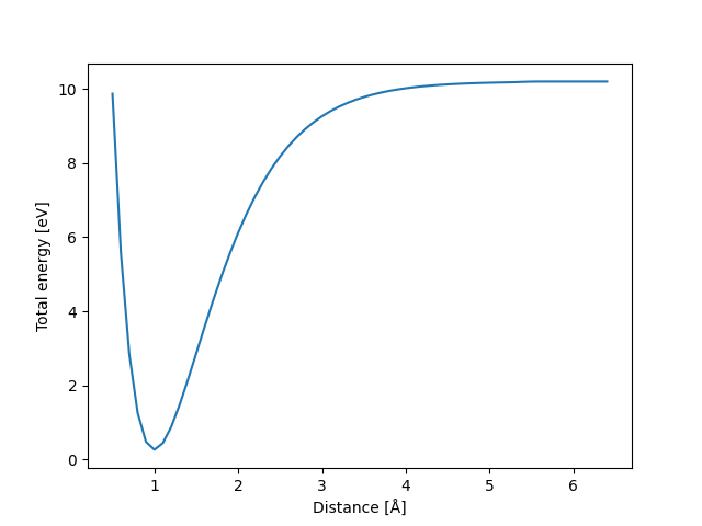
Dissociation energy [eV]: 9.937147312332202