Manipulating Atoms

This tutorial shows how to build and manipulate structures with ASE.

Ag adatom on Ni slab

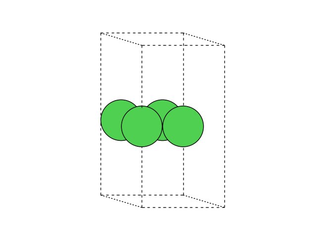
We will set up a one layer slab of four Ni atoms with one Ag adatom. Define the slab atoms:

from math import sqrt

from ase import Atoms

a = 3.55
atoms = Atoms(
    'Ni4',
    cell=[sqrt(2) * a, sqrt(2) * a, 1.0, 90, 90, 120],
    pbc=(1, 1, 0),
    scaled_positions=[(0, 0, 0), (0.5, 0, 0), (0, 0.5, 0), (0.5, 0.5, 0)],
)
atoms.center(vacuum=5.0, axis=2)

Have a look at the cell and positions of the atoms:

print(atoms.cell)

Cell([[5.020458146424487, 0.0, 0.0], [-2.5102290732122423, 4.347844293440141, 0.0], [0.0, 0.0, 10.0]])

print(atoms.positions)

[[ 0.          0.          5.        ]
 [ 2.51022907  0.          5.        ]
 [-1.25511454  2.17392215  5.        ]
 [ 1.25511454  2.17392215  5.        ]]

print(atoms[0])

Atom('Ni', [np.float64(0.0), np.float64(0.0), np.float64(5.0)], index=0)

Visualizing a structure

Write the structure to a file and plot the whole system by bringing up the ase.gui:

from ase.visualize import view
atoms.write('slab.xyz')
view(atoms)

Alternatively, we can plot structures with Matplotlib. Throughout this tutorial, we will be using matplotlib to visualize the structures. Note, however, that in practice using the view function or opening structures in the ase gui directly from the terminal with ase gui structure.xyz gives an interactive view, which might be preferred.

import matplotlib.pyplot as plt

from ase.visualize.plot import plot_atoms

fig, ax = plt.subplots()
plot_atoms(atoms, ax, rotation=('-80x,0y,0z'))
ax.set_axis_off()

Note that we added the rotation argument, so that we can get a side view of the cell.

Repeating a structure

Within the viewer (called ase gui) it is possible to repeat the unit cell in all three directions (using the Repeat ‣ View window). From the command line, use ase gui -r 3,3,2 slab.xyz.

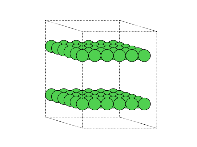
Alternatively, you can also do this directly in ase with the repeat function of the Atoms object.

atoms_repeated = atoms.repeat((3, 3, 2))

This gives a repeated atoms object. We visualize it here again in matplotlib.

fig, ax = plt.subplots()
plot_atoms(atoms_repeated, ax, rotation=('-80x,0y,0z'))
ax.set_axis_off()

Adding atoms

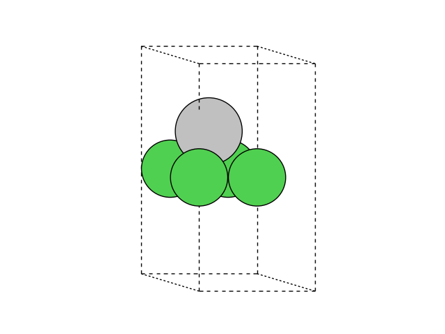
We now add an adatom in a three-fold site at a height of h=1.9 Å: To generate the new positions of the adatom, we are using numpy.

import numpy as np

h = 1.9
relative = (1 / 6, 1 / 6, 0.5)
absolute = np.dot(relative, atoms.cell) + (0, 0, h)
atoms.append('Ag')
atoms.positions[-1] = absolute

The structure now looks like this:

fig, ax = plt.subplots()
plot_atoms(atoms, ax, rotation=('-80x,0y,0z'))
ax.set_axis_off()

Interface building

Now, we will make an interface with Ni(111) and water. First we need a layer of water. One layer of water is constructed in the following script and saved in the file water.traj.

import numpy as np

from ase import Atoms

p = np.array(
    [
        [0.27802511, -0.07732213, 13.46649107],
        [0.91833251, -1.02565868, 13.41456626],
        [0.91865997, 0.87076761, 13.41228287],
        [1.85572027, 2.37336781, 13.56440907],
        [3.13987926, 2.3633134, 13.4327577],
        [1.77566079, 2.37150862, 14.66528237],
        [4.52240322, 2.35264513, 13.37435864],
        [5.16892729, 1.40357034, 13.42661052],
        [5.15567324, 3.30068395, 13.4305779],
        [6.10183518, -0.0738656, 13.27945071],
        [7.3856151, -0.07438536, 13.40814585],
        [6.01881192, -0.08627583, 12.1789428],
    ]
)
c = np.array([[8.490373, 0.0, 0.0], [0.0, 4.901919, 0.0], [0.0, 0.0, 26.93236]])
water = Atoms('4(OH2)', positions=p, cell=c, pbc=[1, 1, 0])
water.write('water.traj')

With the atoms object saved as trajectory file, we can also read the atoms from this file.

from ase.io import read

water = read('water.traj')

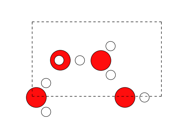
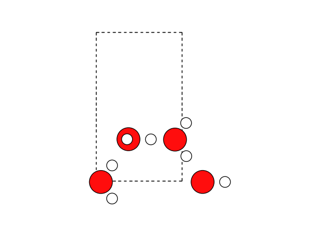
Visualization

Lets take a look at the structure. For this, you can use view to open the ASE gui as show above. Here, we are using matplotlib again.

fig, ax = plt.subplots()
plot_atoms(water, ax)
ax.set_axis_off()

and let’s look at the unit cell.

print(water.cell)

Cell([8.490373, 4.901919, 26.93236])

Creating a Ni slab

We will need a Ni(111) slab which matches the water as closely as possible. A 2x4 orthogonal fcc111 supercell should be good enough.

from ase.build import fcc111

slab = fcc111('Ni', size=[2, 4, 3], a=3.55, orthogonal=True)

fig, ax = plt.subplots()
plot_atoms(slab, ax)
ax.set_axis_off()

print(slab.cell)

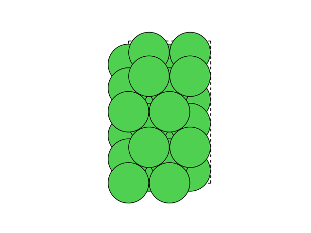
Cell([5.020458146424487, 8.695688586880282, 0.0])

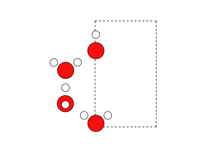
Manipulating a Structure

Looking at the two unit cells, we can see that they match with around 2 percent difference, if we rotate one of the cells 90 degrees in the plane. Let’s rotate the cell:

water.cell = [water.cell[1, 1], water.cell[0, 0], 0.0]

fig, ax = plt.subplots()
plot_atoms(water, ax)
ax.set_axis_off()

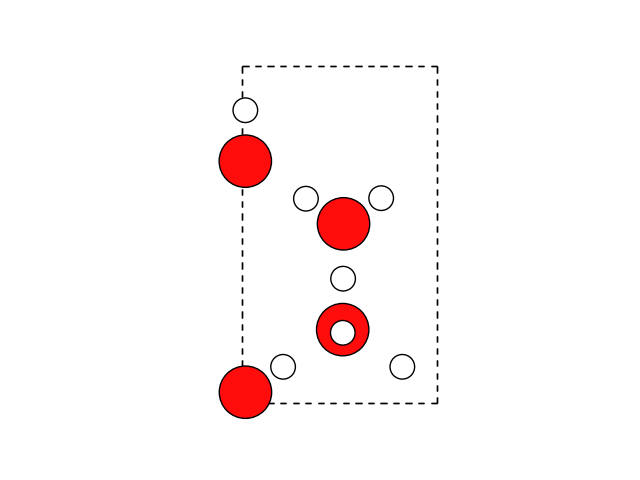
Let’s also rotate() the molecules:

water.rotate(90, 'z', center=(0, 0, 0))

fig, ax = plt.subplots()
plot_atoms(water, ax)
ax.set_axis_off()

Now we can wrap the atoms into the cell

water.wrap()
fig, ax = plt.subplots()
plot_atoms(water, ax)
ax.set_axis_off()

The wrap() method only works if periodic boundary conditions are enabled. We have a 2 percent lattice mismatch between Ni(111) and the water, so we scale the water in the plane to match the cell of the slab. The argument scale_atoms=True indicates that the atomic positions should be scaled with the unit cell. The default is scale_atoms=False indicating that the cartesian coordinates remain the same when the cell is changed.

water.set_cell(slab.cell, scale_atoms=True)
zmin = water.positions[:, 2].min()
zmax = slab.positions[:, 2].max()
water.positions += (0, 0, zmax - zmin + 1.5)

Adding one Structure to the Other

Finally we add the water onto the slab:

interface = slab + water
interface.center(vacuum=6, axis=2)
interface.write('NiH2O.traj')

fig, ax = plt.subplots()
plot_atoms(interface, ax)
ax.set_axis_off()

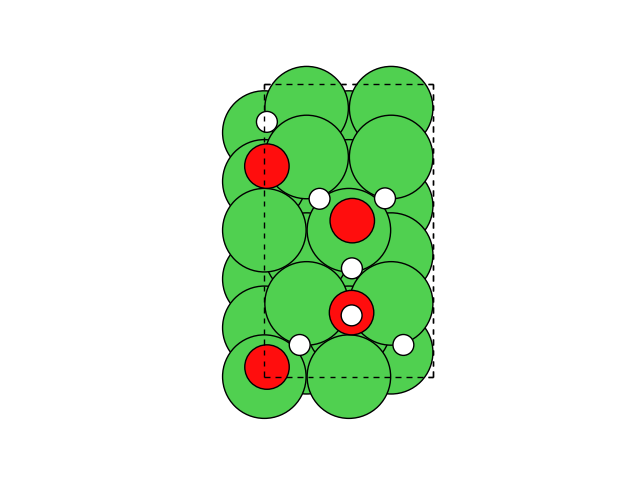
Adding two atoms objects will take the positions from both and the cell and boundary conditions from the first.