Constrained minima hopping (global optimization)

This is an example of a search for a global optimum geometric configuration using the minima hopping algorithm, along with the Hookean class of constraints. This type of approach is useful in searching for the global optimum position of adsorbates on a surface while enforcing that the adsorbates’ identity is preserved. In short, this example searches for a global optimum configuration using the minima hopping algorithm together with Hookean constraints to preserve molecular identity of an adsorbate.

We look for the optimum binding configuration of a \(\mathrm{Cu_2}\) dimer on a fixed Pt(110) surface (Cu/Pt chosen only because EMT supports them). Replace the \(\mathrm{Cu_2}\) dimer with, e.g., CO to find its optimal site while preventing dissociation into separate C and O adsorbates.

Two Hookean constraints are used:

1. Bond-preserving: apply a restorative force if the Cu–Cu distance exceeds 2.6 Å (no force below 2.6 Å), keeping the dimer intact.

2. Keep below plane: apply a downward force if one Cu goes above \(z=15\) Å to avoid the dimer flying off into vacuum.

Outputs. The run writes a text log (hop.log) and a trajectory of accepted minima (minima.traj). You can also visualize progress with the mhsummary.py utility if available.

References

• Minima hopping in ASE usage: ase.optimize.minimahopping (Goedecker, JCP 120, 9911 (2004))

• Hookean constraints: ase.constraints.Hookean

• Constrained minima hopping tutorial page in the ASE docs

Imports and calculator

from __future__ import annotations

import matplotlib.pyplot as plt
import numpy as np

from ase import Atoms
from ase.build import fcc110
from ase.calculators.emt import EMT
from ase.constraints import FixAtoms, Hookean
from ase.io import read
from ase.optimize.minimahopping import MHPlot, MinimaHopping
from ase.visualize.plot import plot_atoms


# Make results reproducible across doc builds. We will pass this random
# number generator to the MinimaHopping algorithm.
seed = 42
rng = np.random.default_rng(seed)

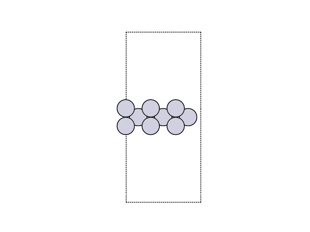
Build a fixed Pt(110) slab

A small slab is enough for the demonstration and keeps CI fast.

slab = fcc110(
    'Pt', size=(3, 2, 3), vacuum=12.0
)  # (x, y, z repeats), ~ few hundred atoms at most
print(slab.pbc)

[ True  True False]

This sets the desired periodic boundary conditions to be periodic in x- and y-direction.

# Fix the whole slab (only the adsorbate will move in this minimal example).
fix = FixAtoms(mask=slab.symbols == 'Pt')
slab.set_constraint(fix)

Now, we can visualize the slab.

fig, ax = plt.subplots()
plot_atoms(slab, ax, rotation=('270x,0y,0z'))
ax.set_axis_off()

We can also attach a calculator.

# Attach an EMT calculator
slab.calc = EMT()

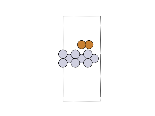
Add a Cu₂ dimer above the surface

Place the dimer roughly above a surface hollow; exact site is not important for the example since minima hopping will explore. Start with a 2.3 Å Cu–Cu distance (near gas-phase value).

top_z = slab.positions[:, 2].max()
cu2 = Atoms('Cu2', positions=[[0.0, 0.0, top_z + 3.0], [2.3, 0.0, top_z + 3.0]])

# Translate laterally to the middle of the cell
cell = slab.get_cell()
xy_center = 0.5 * (cell[0] + cell[1])
cu2.translate([xy_center[0], xy_center[1], 0.0])

atoms = slab + cu2
atoms.calc = EMT()

Now, we can visualize the new structure.

fig, ax = plt.subplots()
plot_atoms(atoms, ax, rotation=('270x,0y,0z'))
ax.set_axis_off()

Hookean constraints

As mentioned above, we want to add two kinds of Hookean constraints:

1. Preserve the Cu–Cu bond if it stretches beyond 2.6 Å: no force for r <= 2.6 Å, Hookean spring k*(r-rt) beyond.

2. Keep one Cu below the plane z = 15 Å using the plane form of Hookean: plane (A,B,C,D) with Ax+By+Cz+D = 0 -> (0,0,1,-15) gives z=15; a downward force is applied if z > 15.

The Hookean API (ASE >= 3.22) accepts:

Hookean(a1, a2, k, rt=None) - a2 can be an atom index, a fixed point (x,y,z), or a plane (A,B,C,D).

Spring constants here are modest to guide but not dominate the dynamics.

i_cu0, i_cu1 = atoms.symbols.search('Cu')

# contraint #1
bond_constraint = Hookean(
    a1=i_cu0, a2=int(i_cu1), k=5.0, rt=2.6
)  # eV/Å^2, threshold 2.6 Å
# contraint #2
z_plane_constraint = Hookean(
    a1=i_cu0, a2=(0.0, 0.0, 1.0, -15.0), k=2.0
)  # plane z=15 Å

atoms.set_constraint([fix, bond_constraint, z_plane_constraint])

Run minima hopping (short demo)

We keep totalsteps small so the example runs quickly in CI. Outputs:

• hop.log: text progress

• minima.traj: accepted local minima

mh = MinimaHopping(
    atoms,
    T0=1500.0,  # initial MD "temperature" (K)
    Ediff0=1.0,  # initial acceptance window (eV)
    mdmin=2,  # MD stop criterion
    logfile='hop.log',
    minima_traj='minima.traj',
    rng=rng,
)

# Run a few steps only for documentation builds.
mh(totalsteps=10)
print(
    'Minima hopping finished.'
    "See 'hop.log' and 'minima.traj' in the working directory."
)

Minima hopping finished.See 'hop.log' and 'minima.traj' in the working directory.

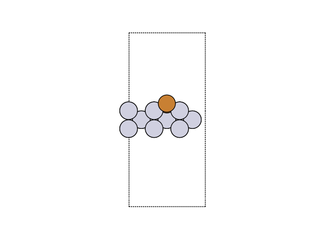
Visualization of Results

Now, we can visualize the new structure. For this we are loading the forth image of the trajectory.

atoms = read('minima.traj')

fig, ax = plt.subplots()
plot_atoms(atoms, ax, rotation=('270x,0y,0z'))
ax.set_axis_off()

We can also analyze this with MHPlot and save the results.

mhplot = MHPlot()
mhplot.save_figure('summary.png')

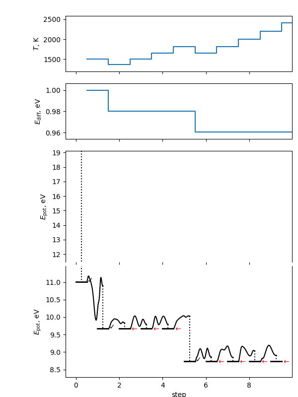
This will make a summary figure, which should see above. As the search is inherently random, yours will look different than this if you used a different random seed (and this will look different each time the documentation is rebuilt). In this figure, you will see on the \(E_\mathrm{pot}\) axes the energy levels of the conformers found. The flat bars represent the energy at the end of each local optimization step. The checkmark indicates the local minimum was accepted; red arrows indicate it was rejected for the three possible reasons. The black path between steps is the potential energy during the molecular dynamics (MD) portion of the step; the dashed line is the local optimization on termination of the MD step. Note the y axis is broken to allow different energy scales between the local minima and the space explored in the MD simulations. The \(T\) and \(E_\mathrm{diff}\) plots show the values of the self-adjusting parameters as the algorithm progresses.

Further Examples

You can find an example of the implementation of this for real adsorbates as well as find suitable parameters for the Hookean constraints:

Andrew Peterson Global optimization of adsorbate–surface structures while preserving molecular identity Top. Catal., Vol. 57, 40 (2014)