
Note
Go to the end to download the full example code.
NEB with IDPP: Image Dependent Pair Potential for improved interpolation of NEB initial guess#
Reference: S. Smidstrup, A. Pedersen, K. Stokbro and H. Jonsson, Improved initial guess for minimum energy path calculations, J. Chem. Phys. 140, 214106 (2014).
Use of the Nudged Elastic Band (NEB) method for transition state search is dependent upon generating an initial guess for the images lying between the initial and final states. The most simple approach is to use linear interpolation of the atomic coordinates. However, this can be problematic as the quality of the interpolated path can ofter be far from the real one. The implication being that a lot of time is spent in the NEB routine optimising the shape of the path, before the transition state is homed-in upon.
The image dependent pair potential (IDPP) is a method that has been developed to provide an improvement to the initial guess for the NEB path. The IDPP method uses the bond distance between the atoms involved in the transition state to create target structures for the images, rather than interpolating the atomic positions. By defining an objective function in terms of the distances between atoms, the NEB algorithm is used with this image dependent pair potential to create the initial guess for the full NEB calculation.
Note
The examples below utilise the EMT calculator for illustrative purposes, the results should not be over interpreted.
This tutorial includes example NEB calculations for two different systems. First, it starts with a simple NEB of Ethane comparing IDPP to the standard linear approach. The second example is for a N atom on a Pt step edge.
Example 1: Ethane#
This example illustrates the use of the IDPP interpolation scheme to generate an initial guess for rotation of a methyl group around the CC bond.
1.1 Generate Initial and Final State#
      Step     Time          Energy          fmax
FIRE:    0 15:30:10        3.078940        4.012422
FIRE:    1 15:30:10        2.530571        3.506100
FIRE:    2 15:30:10        1.950051        2.538108
FIRE:    3 15:30:10        1.752270        1.148539
FIRE:    4 15:30:10        1.732747        1.108297
FIRE:    5 15:30:10        1.696342        1.027750
FIRE:    6 15:30:10        1.648051        0.907203
FIRE:    7 15:30:10        1.594621        0.748189
FIRE:    8 15:30:10        1.543597        0.554845
FIRE:    9 15:30:10        1.502047        0.532019
FIRE:   10 15:30:10        1.475189        0.516589
FIRE:   11 15:30:10        1.465461        0.338747
FIRE:   12 15:30:10        1.465228        0.325538
FIRE:   13 15:30:10        1.464795        0.299554
FIRE:   14 15:30:10        1.464228        0.261663
FIRE:   15 15:30:10        1.463608        0.213166
FIRE:   16 15:30:10        1.463029        0.155784
FIRE:   17 15:30:10        1.462575        0.091667
FIRE:   18 15:30:10        1.462314        0.029444

np.True_
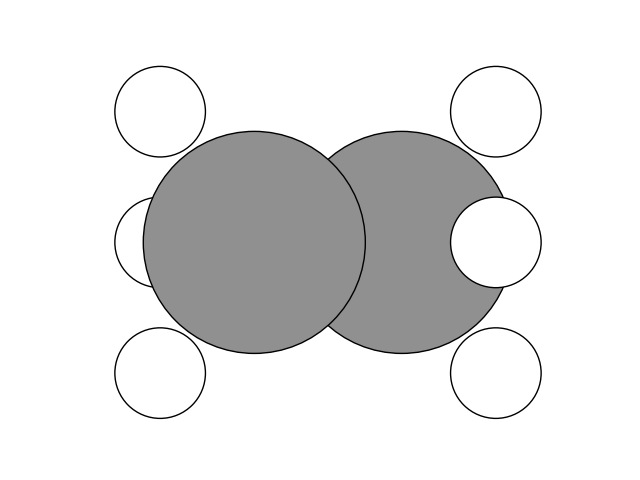
Let’s look at the relaxed molecule.
import matplotlib.pyplot as plt

from ase.visualize.plot import plot_atoms

fig, ax = plt.subplots()
plot_atoms(initial, ax, rotation=('90x,0y,90z'))
ax.set_axis_off()
Now we can create the final state. Since we want to look at the rotation of the methyl group, we switch the position of the Hydrogen atoms on one methyl group. Then, we setup and run the NEB calculation.
final = initial.copy()
final.positions[2:5] = initial.positions[[3, 4, 2]]
1.2 Linear Interpolation Approach#
Generate blank images.
images = [initial]

for i in range(9):
    images.append(initial.copy())
images.append(final)

for image in images:
    image.calc = EMT()


# Run linear interpolation.
neb = NEB(images)
neb.interpolate()

# Run NEB calculation.
qn = FIRE(neb, trajectory='ethane_linear.traj')
qn.run(fmax=0.05)
# You can add a logfile to the FIRE optimizer by adding
# e.g. `logfile='ethane_linear.log` to save the printed output.
/home/ase/.local/lib/python3.13/site-packages/ase/mep/neb.py:329: UserWarning: The default method has changed from 'aseneb' to 'improvedtangent'. The 'aseneb' method is an unpublished, custom implementation that is not recommended as it frequently results in very poor bands. Please explicitly set method='improvedtangent' to silence this warning, or set method='aseneb' if you strictly require the old behavior (results may vary). See: https://gitlab.com/ase/ase/-/merge_requests/3952
  warnings.warn(
      Step     Time          Energy          fmax
FIRE:    0 15:30:10       16.807663       53.427700
FIRE:    1 15:30:10        8.983628       30.051463
FIRE:    2 15:30:10        4.994438       15.778793
FIRE:    3 15:30:10        3.175643        8.523435
FIRE:    4 15:30:10        2.413037        6.022455
FIRE:    5 15:30:10        2.364442        8.524675
FIRE:    6 15:30:11        2.495744       10.615077
FIRE:    7 15:30:11        2.153703        8.124105
FIRE:    8 15:30:11        1.760321        4.244887
FIRE:    9 15:30:11        1.617823        1.151505
FIRE:   10 15:30:11        1.629846        2.986288
FIRE:   11 15:30:11        1.617744        2.835454
FIRE:   12 15:30:11        1.596190        2.542696
FIRE:   13 15:30:11        1.569523        2.125156
FIRE:   14 15:30:11        1.541172        1.606969
FIRE:   15 15:30:11        1.516383        1.018188
FIRE:   16 15:30:11        1.501627        0.581369
FIRE:   17 15:30:11        1.490395        0.502003
FIRE:   18 15:30:11        1.482025        0.834578
FIRE:   19 15:30:11        1.480435        1.295189
FIRE:   20 15:30:11        1.483303        1.589096
FIRE:   21 15:30:11        1.483996        1.634319
FIRE:   22 15:30:12        1.477577        1.397180
FIRE:   23 15:30:12        1.466870        0.879131
FIRE:   24 15:30:12        1.460858        0.264044
FIRE:   25 15:30:12        1.460689        0.260547
FIRE:   26 15:30:12        1.460362        0.253601
FIRE:   27 15:30:12        1.459898        0.243300
FIRE:   28 15:30:12        1.459325        0.229793
FIRE:   29 15:30:12        1.458677        0.213607
FIRE:   30 15:30:12        1.457992        0.195486
FIRE:   31 15:30:12        1.457504        0.175032
FIRE:   32 15:30:12        1.457325        0.150133
FIRE:   33 15:30:12        1.457129        0.120525
FIRE:   34 15:30:12        1.456929        0.102071
FIRE:   35 15:30:12        1.456742        0.133389
FIRE:   36 15:30:12        1.456595        0.150998
FIRE:   37 15:30:12        1.456516        0.143548
FIRE:   38 15:30:12        1.456522        0.104827
FIRE:   39 15:30:12        1.456521        0.102760
FIRE:   40 15:30:13        1.456519        0.098674
FIRE:   41 15:30:13        1.456516        0.092667
FIRE:   42 15:30:13        1.456513        0.084888
FIRE:   43 15:30:13        1.456508        0.075543
FIRE:   44 15:30:13        1.456503        0.064894
FIRE:   45 15:30:13        1.456497        0.053262
FIRE:   46 15:30:13        1.456490        0.046298

np.True_
Using the standard linear interpolation approach, as in the following example, we can see that 47 iterations are required to find the transition state.
1.3 Image Dependent Pair Potential#
However if we modify our script slightly and use the IDPP method to find the initial guess, we can see that the number of iterations required to find the transition state is reduced to 7.
# Optimise molecule.
initial = molecule('C2H6')
initial.calc = EMT()
relax = FIRE(initial, logfile='opt.log')
relax.run(fmax=0.05)

# Create final state.
final = initial.copy()
final.positions[2:5] = initial.positions[[3, 4, 2]]

# Generate blank images.
images = [initial]

for i in range(9):
    images.append(initial.copy())
images.append(final)

for image in images:
    image.calc = EMT()


# Run IDPP interpolation.
neb = NEB(images)
neb.interpolate('idpp')

# Run NEB calculation.
qn = FIRE(neb, trajectory='ethane_idpp.traj')
qn.run(fmax=0.05)
      Step     Time          Energy          fmax
FIRE:    0 15:30:13        1.474291        0.715412
FIRE:    1 15:30:13        1.464595        0.456414
FIRE:    2 15:30:13        1.461252        0.148238
FIRE:    3 15:30:13        1.461159        0.129951
FIRE:    4 15:30:13        1.460988        0.095890
FIRE:    5 15:30:13        1.460768        0.060933
FIRE:    6 15:30:13        1.460533        0.046967

np.True_
Clearly, if one was using a full DFT calculator one can potentially gain a significant time improvement.
Example 2: N Diffusion over a Step Edge#
Often we are interested in generating an initial guess for a surface reaction.
2.1 Generate Initial and Final State#
The first part of this example illustrates how we can optimise our initial and final state structures before using the IDPP interpolation to generate our initial guess for the NEB calculation:
import numpy as np
from ase import Atoms
from ase.calculators.emt import EMT
from ase.constraints import FixAtoms
from ase.lattice.cubic import FaceCenteredCubic
from ase.mep import NEB
from ase.optimize.fire import FIRE as FIRE
# Set the number of images you want.
nimages = 5
# Some algebra to determine surface normal and the plane of the surface.
d3 = [2, 1, 1]
a1 = np.array([0, 1, 1])
d1 = np.cross(a1, d3)
a2 = np.array([0, -1, 1])
d2 = np.cross(a2, d3)
# Create the slab.
slab = FaceCenteredCubic(
directions=[d1, d2, d3], size=(2, 1, 2), symbol=('Pt'), latticeconstant=3.9
)
# Add some vacuum to the slab.
uc = slab.get_cell()
uc[2] += [0.0, 0.0, 10.0] # There are ten layers of vacuum.
uc = slab.set_cell(uc, scale_atoms=False)
# Some positions needed to place the atom in the correct place.
x1 = 1.379
x2 = 4.137
x3 = 2.759
y1 = 0.0
y2 = 2.238
z1 = 7.165
z2 = 6.439
# Add the adatom to the list of atoms and set constraints of surface atoms.
slab += Atoms('N', [((x2 + x1) / 2, y1, z1 + 1.5)])
FixAtoms(mask=slab.symbols == 'Pt')
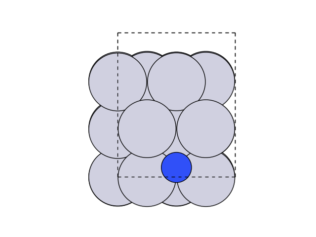
# Optimise the initial state: atom below step.
initial = slab.copy()
initial.calc = EMT()
relax = FIRE(initial, logfile='opt.log')
relax.run(fmax=0.05)
np.True_
Now let’s visualize this.
fig, ax = plt.subplots()
plot_atoms(initial, ax, rotation=('0x,0y,0z'))
ax.set_axis_off()
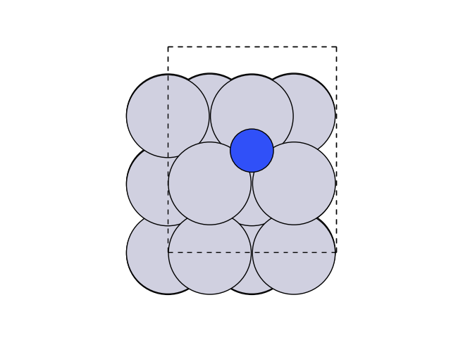
We can now create and optimise the final state by moving the atom above the step.
np.True_
Now let’s visualize this.
fig, ax = plt.subplots()
plot_atoms(final, ax, rotation=('0x,0y,0z'))
ax.set_axis_off()
2.2 Image Dependent Pair Potential#
Now we are ready to setup the NEB with the IDPP interpolation.
# Create a list of images for interpolation.
images = [initial]
for i in range(nimages):
    images.append(initial.copy())

for image in images:
    image.calc = EMT()

images.append(final)

# Carry out idpp interpolation.
neb = NEB(images)
neb.interpolate('idpp')

# Run NEB calculation.
qn = FIRE(neb, trajectory='N_diffusion.traj')
qn.run(fmax=0.05)
      Step     Time          Energy          fmax
FIRE:    0 15:30:15        4.894646        5.113621
FIRE:    1 15:30:15        4.596641        3.666279
FIRE:    2 15:30:15        4.297856        1.781956
FIRE:    3 15:30:15        4.118322        2.113806
FIRE:    4 15:30:15        4.033812        1.577100
FIRE:    5 15:30:15        4.019813        1.461991
FIRE:    6 15:30:15        3.995645        1.245666
FIRE:    7 15:30:15        3.967646        0.953102
FIRE:    8 15:30:15        3.943934        0.617335
FIRE:    9 15:30:15        3.927608        0.438807
FIRE:   10 15:30:15        3.916445        0.685649
FIRE:   11 15:30:15        3.910612        0.882394
FIRE:   12 15:30:16        3.904533        0.976873
FIRE:   13 15:30:16        3.893976        0.935090
FIRE:   14 15:30:16        3.880874        0.771322
FIRE:   15 15:30:16        3.869786        0.440124
FIRE:   16 15:30:16        3.861905        0.340737
FIRE:   17 15:30:16        3.857292        0.465015
FIRE:   18 15:30:16        3.856022        0.439083
FIRE:   19 15:30:16        3.854481        0.388949
FIRE:   20 15:30:16        3.852588        0.318015
FIRE:   21 15:30:16        3.850678        0.231496
FIRE:   22 15:30:16        3.849069        0.137381
FIRE:   23 15:30:16        3.847949        0.116435
FIRE:   24 15:30:16        3.847292        0.169711
FIRE:   25 15:30:16        3.846866        0.220639
FIRE:   26 15:30:16        3.846818        0.217252
FIRE:   27 15:30:16        3.846725        0.210553
FIRE:   28 15:30:16        3.846591        0.200692
FIRE:   29 15:30:16        3.846423        0.187893
FIRE:   30 15:30:16        3.846230        0.172458
FIRE:   31 15:30:16        3.846021        0.154759
FIRE:   32 15:30:16        3.845804        0.135248
FIRE:   33 15:30:16        3.845565        0.112200
FIRE:   34 15:30:16        3.845311        0.085865
FIRE:   35 15:30:17        3.845050        0.062334
FIRE:   36 15:30:17        3.844785        0.060819
FIRE:   37 15:30:17        3.844509        0.084548
FIRE:   38 15:30:17        3.844200        0.103352
FIRE:   39 15:30:17        3.843830        0.113475
FIRE:   40 15:30:17        3.843374        0.111870
FIRE:   41 15:30:17        3.842832        0.096360
FIRE:   42 15:30:17        3.842246        0.066624
FIRE:   43 15:30:17        3.841691        0.039643

np.True_
2.3 Linear Interpolation Approach#
To again illustrate the potential speedup, the following script uses the linear interpolation. This takes more iterations to find a transition state, compared to using the IDPP interpolation. We start from the initial and final state we generated above.
# Create a list of images for interpolation.
images = [initial]
for i in range(nimages):
    images.append(initial.copy())

for image in images:
    image.calc = EMT()

images.append(final)

# Carry out linear interpolation.
neb = NEB(images)
neb.interpolate()

# Run NEB calculation.
qn = FIRE(neb, trajectory='N_diffusion_lin.traj')
qn.run(fmax=0.05)
      Step     Time          Energy          fmax
FIRE:    0 15:30:17        9.597339       18.109950
FIRE:    1 15:30:17        6.490830       10.803819
FIRE:    2 15:30:17        5.049471        5.744292
FIRE:    3 15:30:17        4.701493        2.784721
FIRE:    4 15:30:17        4.890363        6.197566
FIRE:    5 15:30:17        4.687247        5.010258
FIRE:    6 15:30:17        4.417183        3.162095
FIRE:    7 15:30:17        4.221940        1.593666
FIRE:    8 15:30:17        4.147916        2.251744
FIRE:    9 15:30:17        4.140625        2.680253
FIRE:   10 15:30:17        4.124519        2.701390
FIRE:   11 15:30:17        4.072074        2.304749
FIRE:   12 15:30:18        3.993095        1.513131
FIRE:   13 15:30:18        3.931022        0.761804
FIRE:   14 15:30:18        3.924567        0.642927
FIRE:   15 15:30:18        3.922907        0.636018
FIRE:   16 15:30:18        3.919699        0.622303
FIRE:   17 15:30:18        3.915156        0.601975
FIRE:   18 15:30:18        3.909574        0.575304
FIRE:   19 15:30:18        3.903305        0.542624
FIRE:   20 15:30:18        3.896721        0.504321
FIRE:   21 15:30:18        3.890175        0.460825
FIRE:   22 15:30:18        3.883339        0.417934
FIRE:   23 15:30:18        3.876605        0.364215
FIRE:   24 15:30:18        3.870376        0.296742
FIRE:   25 15:30:18        3.864959        0.254417
FIRE:   26 15:30:18        3.860555        0.306728
FIRE:   27 15:30:18        3.857397        0.312943
FIRE:   28 15:30:18        3.855789        0.272507
FIRE:   29 15:30:18        3.855522        0.219988
FIRE:   30 15:30:18        3.855201        0.258925
FIRE:   31 15:30:18        3.852933        0.250428
FIRE:   32 15:30:18        3.848467        0.189390
FIRE:   33 15:30:19        3.844307        0.115960
FIRE:   34 15:30:19        3.843091        0.121178
FIRE:   35 15:30:19        3.842864        0.110985
FIRE:   36 15:30:19        3.842468        0.091936
FIRE:   37 15:30:19        3.841999        0.070254
FIRE:   38 15:30:19        3.841555        0.061877
FIRE:   39 15:30:19        3.841199        0.052204
FIRE:   40 15:30:19        3.840936        0.056882
FIRE:   41 15:30:19        3.840723        0.065668
FIRE:   42 15:30:19        3.840496        0.061557
FIRE:   43 15:30:19        3.840256        0.044569

np.True_