Partly occupied Wannier Functions

This tutorial walks through building partly occupied Wannier functions with the ase.dft.wannier module and the GPAW electronic structure code. For more information on the details of the method and the implementation, see

K. S. Thygesen, L. B. Hansen, and K. W. Jacobsen

Partly occupied Wannier functions: Construction and applications

Phys. Rev. B 72, 125119 (2005)

Benzene molecule

Step 1 – Ground-state calculation

Run the script below to obtain the ground-state density and the Kohn–Sham (KS) orbitals. The result is stored in benzene.gpw.

import matplotlib.pyplot as plt
import numpy as np
from gpaw import GPAW, restart

from ase import Atoms
from ase.build import molecule
from ase.dft.kpoints import monkhorst_pack
from ase.dft.wannier import Wannier

atoms = molecule('C6H6')
atoms.center(vacuum=3.5)

calc = GPAW(mode='pw', xc='PBE', txt='benzene.txt', nbands=18)
atoms.calc = calc
atoms.get_potential_energy()

calc = calc.fixed_density(
    txt='benzene-harris.txt',
    nbands=40,
    convergence={'bands': 35},
)
atoms.get_potential_energy()

calc.write('benzene.gpw', mode='all')

Step 2 – Maximally localized WFs for the occupied subspace (15 WFs)

There are 15 occupied bands in the benzene molecule. We construct one Wannier function per occupied band by setting nwannier = 15. By calling wan.localize(), the code attempts to minimize the spread functional using a gradient-descent algorithm. The resulting WFs are written to .cube files, which allows them to be inspected using e.g. VESTA.

atoms, calc = restart('benzene.gpw', txt=None)

# Make wannier functions of occupied space only
wan = Wannier(nwannier=15, calc=calc)
wan.localize()
for i in range(wan.nwannier):
    wan.write_cube(i, f'benzene15_{i}.cube')

Step 3 – Adding three extra degrees of freedom (18 WFs)

To improve localization we augment the basis with three extra Wannier functions - so-called extra degrees of freedom (nwannier = 18, fixedstates = 15). This will allow the Wannierization procedure to use the unoccupied states to minimize spread functional.

atoms, calc = restart('benzene.gpw', txt=None)

# Make wannier functions using (three) extra degrees of freedom.
wan = Wannier(nwannier=18, calc=calc, fixedstates=15)
wan.localize()
wan.save('wan18.json')
for i in range(wan.nwannier):
    wan.write_cube(i, f'benzene18_{i}.cube')

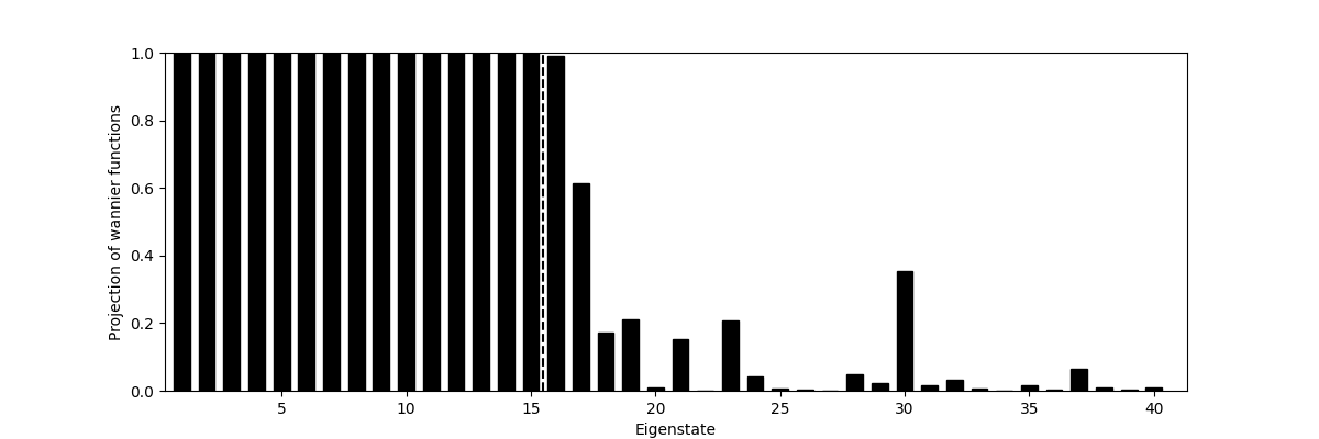
Step 4 – Spectral-weight analysis

The script below projects the WFs on the KS eigenstates. You should see the 15 lowest bands perfectly reconstructed (weight ≃ 1.0) while higher bands are only partially represented.

atoms, calc = restart('benzene.gpw', txt=None)
wan = Wannier(nwannier=18, calc=calc, fixedstates=15, file='wan18.json')

weight_n = np.sum(abs(wan.V_knw[0]) ** 2, 1)
N = len(weight_n)
F = wan.fixedstates_k[0]
plt.figure(1, figsize=(12, 4))
plt.bar(
    range(1, N + 1),
    weight_n,
    width=0.65,
    bottom=0,
    color='k',
    edgecolor='k',
    linewidth=None,
    align='center',
    orientation='vertical',
)
plt.plot([F + 0.5, F + 0.5], [0, 1], 'k--')
plt.axis(xmin=0.32, xmax=N + 1.33, ymin=0, ymax=1)
plt.xlabel('Eigenstate')
plt.ylabel('Projection of wannier functions')
plt.savefig('spectral_weight.png')
plt.show()

Polyacetylene chain (1-D periodic)

We now want to construct partially occupied Wannier functions to describe a polyacetylene chain.

Step 1 – Structure & ground-state calculation

Polyacetylene is modelled as an infinite chain; we therefore enable periodic boundary conditions along x.

kpts = monkhorst_pack((13, 1, 1))
calc = GPAW(
    mode='pw',
    xc='PBE',
    kpts=kpts,
    nbands=12,
    txt='poly.txt',
    convergence={'bands': 9},
    symmetry='off',
)

CC = 1.38
CH = 1.094
a = 2.45
x = a / 2.0
y = np.sqrt(CC**2 - x**2)
atoms = Atoms(
    'C2H2',
    pbc=(True, False, False),
    cell=(a, 8.0, 6.0),
    calculator=calc,
    positions=[[0, 0, 0], [x, y, 0], [x, y + CH, 0], [0, -CH, 0]],
)
atoms.center()
atoms.get_potential_energy()
calc.write('poly.gpw', mode='all')

Step 2 – Wannierization

We repeat the localization procedure, keeping the five lowest bands fixed and adding one extra degree of freedom to aid localization.

import numpy as np
from gpaw import restart

from ase.dft.wannier import Wannier

atoms, calc = restart('poly.gpw', txt=None)

# Make wannier functions using (one) extra degree of freedom
wan = Wannier(
    nwannier=6,
    calc=calc,
    fixedenergy=1.5,
    initialwannier='orbitals',
    functional='var',
)
wan.localize()
wan.save('poly.json')
wan.translate_all_to_cell((2, 0, 0))
for i in range(wan.nwannier):
    wan.write_cube(i, f'polyacetylene_{i}.cube')

# Print Kohn-Sham bandstructure
ef = calc.get_fermi_level()
with open('KSbands.txt', 'w') as fd:
    for k, kpt_c in enumerate(calc.get_ibz_k_points()):
        for eps in calc.get_eigenvalues(kpt=k):
            print(kpt_c[0], eps - ef, file=fd)

# Print Wannier bandstructure
with open('WANbands.txt', 'w') as fd:
    for k in np.linspace(-0.5, 0.5, 100):
        ham = wan.get_hamiltonian_kpoint([k, 0, 0])
        for eps in np.linalg.eigvalsh(ham).real:
            print(k, eps - ef, file=fd)

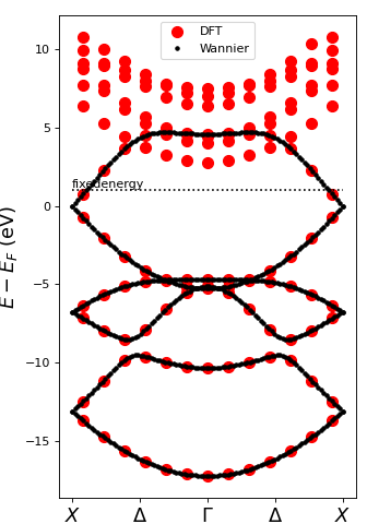
Step 3 – High-resolution band structure

Using the Wannier Hamiltonian we can interpolate the band structure on a fine 100-point k mesh and compare it to the original DFT result.

fig = plt.figure(dpi=80, figsize=(4.2, 6))
fig.subplots_adjust(left=0.16, right=0.97, top=0.97, bottom=0.05)

# Plot KS bands
k, eps = np.loadtxt('KSbands.txt', unpack=True)
plt.plot(k, eps, 'ro', label='DFT', ms=9)

# Plot Wannier bands
k, eps = np.loadtxt('WANbands.txt', unpack=True)
plt.plot(k, eps, 'k.', label='Wannier')

plt.plot([-0.5, 0.5], [1, 1], 'k:', label='_nolegend_')
plt.text(-0.5, 1, 'fixedenergy', ha='left', va='bottom')
plt.axis('tight')
plt.xticks(
    [-0.5, -0.25, 0, 0.25, 0.5],
    [r'$X$', r'$\Delta$', r'$\Gamma$', r'$\Delta$', r'$X$'],
    size=16,
)
plt.ylabel(r'$E - E_F\  \rm{(eV)}$', size=16)
plt.legend()
plt.savefig('bands.png', dpi=80)
plt.show()

Within the fixed-energy window—that is, for energies below the fixed-energy line—the Wannier-interpolated bands coincide perfectly with the DFT reference (red circles). Above this window the match is lost, because the degrees of freedom deliberately mix several Kohn–Sham states to achieve maximal real-space localisation.