Nanoparticle

This tutorial shows how to use the ase.cluster module to set up metal nanoparticles with common crystal forms. Please have a quick look at the module’s documentation linked above.

Build and optimise nanoparticle

Consider ase.cluster.Octahedron(). Aside from generating strictly octahedral nanoparticles, it also offers a cutoff keyword to cut the corners of the octahedron. This produces “truncated octahedra”, a well-known structural motif in nanoparticles. Also, the lattice will be consistent with the bulk FCC structure of silver.

Exercise

Play around with ase.cluster.Octahedron() to produce truncated octahedra. Here we set up a cuboctahedral silver nanoparticle with 55 atoms. As always, verify yourself with the ASE GUI that it is beautiful.

from ase.cluster import Octahedron

atoms = Octahedron('Ag', 5, cutoff=2)

ASE provides a forcefield code based on effective medium theory, ase.calculators.emt.EMT, which works for the FCC metals (Cu, Ag, Au, Pt, and friends). This is much faster than DFT so let’s use it to optimise our cuboctahedron.

from ase.calculators.emt import EMT
from ase.optimize import BFGS

atoms.calc = EMT()
opt = BFGS(atoms, trajectory='opt.traj')
has_converged = opt.run(fmax=0.01)

      Step     Time          Energy          fmax
BFGS:    0 23:38:44       20.334210        0.801013
BFGS:    1 23:38:44       20.147034        0.751003
BFGS:    2 23:38:44       19.301247        0.678888
BFGS:    3 23:38:44       19.196190        0.375474
BFGS:    4 23:38:44       19.155598        0.352885
BFGS:    5 23:38:44       18.907350        0.127899
BFGS:    6 23:38:44       18.893453        0.056286
BFGS:    7 23:38:44       18.891833        0.053418
BFGS:    8 23:38:44       18.886078        0.049818
BFGS:    9 23:38:44       18.882155        0.037683
BFGS:   10 23:38:44       18.880054        0.022328
BFGS:   11 23:38:44       18.879700        0.016541
BFGS:   12 23:38:44       18.879541        0.013518
BFGS:   13 23:38:44       18.879298        0.011513
BFGS:   14 23:38:44       18.879077        0.009199

Ground state

One of the most interesting questions of metal nanoparticles is how their electronic structure and other properties depend on size. A small nanoparticle is like a molecule with just a few discrete energy levels. A large nanoparticle is like a bulk material with a continuous density of states. Let’s calculate the Kohn–Sham spectrum (and density of states) of our nanoparticle.

We set up a GPAW calculator and as usual, we set a few parameters to save time since this is not a real production calculation. We want a smaller basis set and also a PAW dataset with fewer electrons than normal. We also want to use Fermi smearing since there could be multiple electronic states near the Fermi level. These are GPAW-specific keywords — with another code, those variables would have other names.

from gpaw import GPAW, FermiDirac

from ase.io import read

atoms = read('opt.traj')

calc = GPAW(
    mode='lcao',
    basis='sz(dzp)',
    txt='gpaw.txt',
    occupations=FermiDirac(0.1),
    setups={'Ag': '11'},
)

We use this calculator to run a single-point calculation on the optimised silver cluster. After the calculation, we dump the ground state to a file, to be reused later.

atoms.calc = calc
atoms.center(vacuum=4.0)
atoms.get_potential_energy()
atoms.calc.write('groundstate.gpw')

Density of states

Once we have saved the .gpw file, we can write a new script which loads it and gets the DOS:

import matplotlib.pyplot as plt

from ase.dft.dos import DOS

calc = GPAW('groundstate.gpw')
dos = DOS(calc, npts=800, width=0.1)
energies = dos.get_energies()
weights = dos.get_dos()
efermi = calc.get_fermi_level()

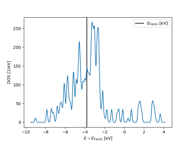
In this example, we sample the DOS using Gaussians of width 0.1 eV. We also mark the Fermi level in the plot.

fig, ax = plt.subplots()
ax.axvline(efermi, color='k', label=r'$E_{\mathrm{Fermi}}$ [eV]')
ax.plot(energies, weights)
ax.set_xlabel(r'$E - E_{\mathrm{Fermi}}$ [eV]')
ax.set_ylabel('DOS [1/eV]')
ax.legend()
plt.show()

Exercise

Looking at the plot, is this spectrum best understood as continuous or discrete?

The graph should show us that already with 55 atoms, the plentiful d electrons are well on their way to forming a continuous band (recall we are using 0.1 eV Gaussian smearing). Meanwhile the energies of the few s electrons split over a wider range, and we clearly see isolated peaks: The s states are still clearly quantized and have significant gaps. What characterises the noble metals Cu, Ag, and Au, is that their d band is fully occupied so that the Fermi level lies among these s states. Clusters with a different number of electrons might have higher or lower Fermi level, strongly affecting their reactivity. We can conjecture that at 55 atoms, the properties of free-standing Ag nanoparticles are probably strongly size dependent.

The above analysis is speculative. To verify the analysis we would want to calculate s, p, and d-projected DOS to see if our assumptions were correct. In case we want to go on doing this, the GPAW documentation will be of help, see: GPAW DOS.