Calculating Delta-values

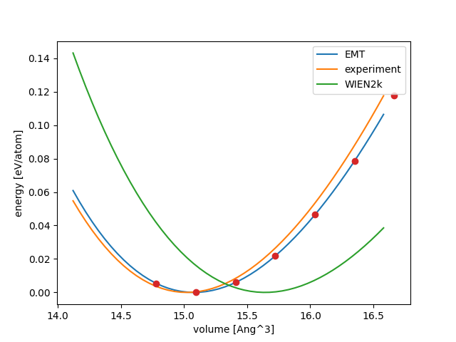
In this tutorial we compare the equation-of-state (EOS) calculated for 7 FCC metals using values from EMT, WIEN2k and experiment. Each EOS is described by three parameters:

• volume per atom

• bulk modulus

• pressure derivative of the bulk modulus

Differences between two EOS’s can be measured by a single \(\Delta\) value defined as:

\[\Delta = \sqrt{\frac{\int_{V_a}^{V_b} \left( E_1(V) - E_2(V) \right)^2 \, dV}{V_b - V_a}}\]

where \(E_n(V)\) is the energy per atom as a function of volume. The \(\Delta\) value can be calculated using the ase.utils.deltacodesdft.delta() function:

ase.utils.deltacodesdft.delta(v1: float, B1: float, Bp1: float, v2: float, B2: float, Bp2: float, symmetric=True) → float

Calculate Delta-value between two equation of states.

See also

molmod/DeltaCodesDFT

Parameters:

• v1 (float) – Volume per atom.

• v2 (float) – Volume per atom.

• B1 (float) – Bulk-modulus (in eV/Ang^3).

• B2 (float) – Bulk-modulus (in eV/Ang^3).

• Bp1 (float) – Pressure derivative of bulk-modulus.

• Bp2 (float) – Pressure derivative of bulk-modulus.

• symmetric (bool) – Default is to calculate a symmetric delta.

Returns:

delta – Delta value in eV/atom.

Return type:

float

See also

• Collection of ground-state elemental crystals: DeltaCodesDFT

• Equation-of-state module: ase.eos

We get the WIEN2k and experimental numbers from the DeltaCodesDFT ASE-collection and we calculate the EMT EOS using this script:

from pathlib import Path

import numpy as np

from ase.calculators.emt import EMT
from ase.collections import dcdft
from ase.io import Trajectory

trajfiles = []

for symbol in ['Al', 'Ni', 'Cu', 'Pd', 'Ag', 'Pt', 'Au']:
    trajfile = Path(f'{symbol}.traj')
    with Trajectory(trajfile, 'w') as traj:
        for s in range(94, 108, 2):
            atoms = dcdft[symbol]
            atoms.set_cell(atoms.cell * (s / 100) ** (1 / 3), scale_atoms=True)
            atoms.calc = EMT()
            atoms.get_potential_energy()
            traj.write(atoms)
    trajfiles.append(trajfile)

And fit to a Birch-Murnaghan EOS:

import json

from ase.eos import EquationOfState as EOS
from ase.io import read


def fit(symbol: str) -> tuple[float, float, float, float]:
    V = []
    E = []
    for atoms in read(f'{symbol}.traj@:'):
        V.append(atoms.get_volume() / len(atoms))
        E.append(atoms.get_potential_energy() / len(atoms))

    eos = EOS(V, E, 'birchmurnaghan')
    eos.fit(warn=False)
    e0, B, Bp, v0 = eos.eos_parameters
    return e0, v0, B, Bp


data = {}  # Dict[str, Dict[str, float]]
for path in trajfiles:
    symbol = path.stem
    e0, v0, B, Bp = fit(symbol)
    data[symbol] = {
        'emt_energy': e0,
        'emt_volume': v0,
        'emt_B': B,
        'emt_Bp': Bp,
    }

Path('fit.json').write_text(json.dumps(data))

964

Result for Pt using EMT:

import matplotlib.pyplot as plt

V, E = [], []
for atoms in read('Pt.traj@:'):
    V.append(atoms.get_volume() / len(atoms))
    E.append(atoms.get_potential_energy() / len(atoms))

eos = EOS(V, E, 'birchmurnaghan')
eos.fit(warn=False)

fig = plt.figure()
ax = fig.gca()
eos.plot(ax=ax)  # draw onto the current axes
ax.set_xlim(14.0, 16.0)
ax.set_xlabel('volume [Å^3/atom]')
ax.set_ylabel('energy [eV/atom]')
plt.tight_layout()

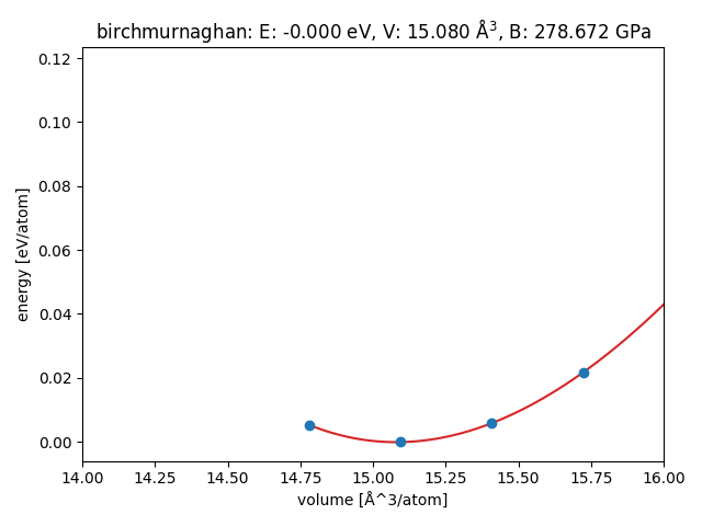
Result for Pt using EMT compared to experiment and WIEN2k Equilibrium volumes (Å^3/atom):

symbol	emt	exp	wien2k
Pt	15.08	15.02	15.64
Al	15.93	16.27	16.48
Ni	10.60	10.81	10.89
Au	16.68	16.82	17.97
Pd	14.59	14.56	15.31
Ag	16.77	16.85	17.85
Cu	11.57	11.65	11.95

Bulk moduli in GPa:

:header: symbol, emt, exp, wien2k

Pt	278.67	285.51	248.71
Al	39.70	77.14	78.08
Ni	176.23	192.46	200.37
Au	174.12	182.01	139.11
Pd	180.43	187.19	168.63
Ag	100.06	105.71	90.15
Cu	134.41	144.28	141.33

Pressure derivative of bulk-moduli:

:header: symbol, emt, exp, wien2k

Pt	5.31	5.18	5.46
Al	2.72	4.45	4.57
Ni	3.76	4.00	5.00
Au	5.46	6.40	5.76
Pd	5.17	5.00	5.56
Ag	4.75	4.72	5.42
Cu	4.21	4.88	4.86

Now, we can calculate \(\Delta\) between EMT and WIEN2k for Pt:

from ase.units import kJ
from ase.utils.deltacodesdft import delta

delta(15.08, 278.67 * 1e-24 * kJ, 5.31, 15.64, 248.71 * 1e-24 * kJ, 5.46)

np.float64(0.03205389052984122)

Here are all the \(\Delta\) values (in meV/atom) calculated with the script below:

:header: symbol, emt-exp, emt-wien2k, exp-wien2k

Pt	3.5	32.2	35.9
Al	5.9	8.6	3.6
Ni	8.6	12.5	3.7
Au	5.9	43.7	39.4
Pd	1.0	27.6	29.0
Ag	1.9	22.4	21.3
Cu	2.7	11.9	9.5

from ase.eos import birchmurnaghan

# Read EMT data:
data = json.loads(Path('fit.json').read_text())
# Insert values from experiment and WIEN2k:
for symbol in data:
    dcdft_dct = dcdft.data[symbol]
    dcdft_dct['exp_B'] *= 1e-24 * kJ
    dcdft_dct['wien2k_B'] *= 1e-24 * kJ
    data[symbol].update(dcdft_dct)

for name in ['volume', 'B', 'Bp']:
    with open(name + '.csv', 'w') as fd:
        print('# symbol, emt, exp, wien2k', file=fd)
        for symbol, dct in data.items():
            values = [
                dct[code + '_' + name] for code in ['emt', 'exp', 'wien2k']
            ]
            if name == 'B':
                values = [val * 1e24 / kJ for val in values]
            print(
                f'{symbol},',
                ', '.join(f'{value:.2f}' for value in values),
                file=fd,
            )

with open('delta.csv', 'w') as fd:
    print('# symbol, emt-exp, emt-wien2k, exp-wien2k', file=fd)
    for symbol, dct in data.items():
        # Get v0, B, Bp:
        emt, exp, wien2k = (
            (dct[code + '_volume'], dct[code + '_B'], dct[code + '_Bp'])
            for code in ['emt', 'exp', 'wien2k']
        )
        print(
            f'{symbol}, {delta(*emt, *exp) * 1000:.1f}, '
            f'{delta(*emt, *wien2k) * 1000:.1f}, '
            f'{delta(*exp, *wien2k) * 1000:.1f}',
            file=fd,
        )

        if symbol == 'Pt':
            va = min(emt[0], exp[0], wien2k[0])
            vb = max(emt[0], exp[0], wien2k[0])
            v = np.linspace(0.94 * va, 1.06 * vb)
            for (v0, B, Bp), code in [
                (emt, 'EMT'),
                (exp, 'experiment'),
                (wien2k, 'WIEN2k'),
            ]:
                plt.plot(v, birchmurnaghan(v, 0.0, B, Bp, v0), label=code)
            e0 = dct['emt_energy']
            V = []
            E = []
            for atoms in read('Pt.traj@:'):
                V.append(atoms.get_volume() / len(atoms))
                E.append(atoms.get_potential_energy() / len(atoms) - e0)
            plt.plot(V, E, 'o')
            plt.legend()
            plt.xlabel('volume [Ang^3]')
            plt.ylabel('energy [eV/atom]')
            plt.savefig('Pt.png')