Note

Go to the end to download the full example code.

Surface diffusion energy barriers using the Nudged Elastic Band (NEB) method#

import matplotlib.pyplot as plt

from ase.build import add_adsorbate, fcc100
from ase.calculators.emt import EMT
from ase.constraints import FixAtoms
from ase.io import read
from ase.mep import NEB
from ase.optimize import BFGS, QuasiNewton
from ase.parallel import world
from ase.visualize.plot import plot_atoms

First, set up the initial and final states: 2x2-Al(001) surface with 3 layers and an Au atom adsorbed in a hollow site:

slab = fcc100('Al', size=(2, 2, 3))
add_adsorbate(slab, 'Au', 1.7, 'hollow')
slab.center(axis=2, vacuum=4.0)

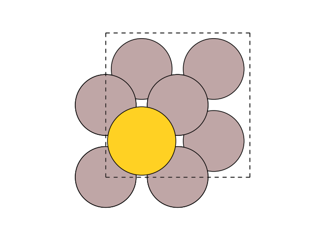
Make sure the structure is correct:

fig, ax = plt.subplots()
plot_atoms(slab, ax)
ax.set_axis_off()

Fix second and third layers:

mask = [atom.tag > 1 for atom in slab]
print(mask)
slab.set_constraint(FixAtoms(mask=mask))

[np.True_, np.True_, np.True_, np.True_, np.True_, np.True_, np.True_, np.True_, np.False_, np.False_, np.False_, np.False_, np.False_]

Use EMT potential:

slab.calc = EMT()

Initial state:

qn = QuasiNewton(slab, trajectory='initial.traj')
qn.run(fmax=0.05)

                Step[ FC]     Time          Energy          fmax
BFGSLineSearch:    0[  0] 15:12:52        3.323870       0.2462
BFGSLineSearch:    1[  1] 15:12:52        3.314754       0.0378

np.True_

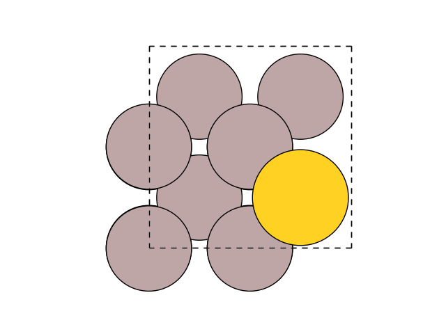
Final state:

slab[-1].x += slab.get_cell()[0, 0] / 2
qn = QuasiNewton(slab, trajectory='final.traj')
qn.run(fmax=0.05)

                Step[ FC]     Time          Energy          fmax
BFGSLineSearch:    0[  0] 15:12:52        3.320051       0.1208
BFGSLineSearch:    1[  1] 15:12:52        3.316117       0.0474

np.True_

Note

Notice how the tags are used to select the constrained atoms

Now, do the NEB calculation:

initial = read('initial.traj')
final = read('final.traj')

constraint = FixAtoms(mask=[atom.tag > 1 for atom in initial])

images = [initial]
for i in range(3):
    image = initial.copy()
    image.calc = EMT()
    image.set_constraint(constraint)
    images.append(image)

images.append(final)

neb = NEB(images, method='improvedtangent')
neb.interpolate()
qn = BFGS(neb, trajectory='neb.traj')
qn.run(fmax=0.05)

      Step     Time          Energy          fmax
BFGS:    0 15:12:52        4.219952        3.520752
BFGS:    1 15:12:52        3.937039        2.176460
BFGS:    2 15:12:52        3.719814        0.435144
BFGS:    3 15:12:52        3.709652        0.230134
BFGS:    4 15:12:52        3.708878        0.244118
BFGS:    5 15:12:52        3.706087        0.257725
BFGS:    6 15:12:52        3.698531        0.213294
BFGS:    7 15:12:52        3.692120        0.246238
BFGS:    8 15:12:52        3.692278        0.187553
BFGS:    9 15:12:52        3.693494        0.172952
BFGS:   10 15:12:52        3.692670        0.151720
BFGS:   11 15:12:52        3.690813        0.073884
BFGS:   12 15:12:52        3.690200        0.071211
BFGS:   13 15:12:52        3.690380        0.078122
BFGS:   14 15:12:52        3.690427        0.103668
BFGS:   15 15:12:52        3.689897        0.100381
BFGS:   16 15:12:52        3.689034        0.055057
BFGS:   17 15:12:52        3.688737        0.028898

np.True_

Visualize the results with:

.. GENERATED FROM PYTHON SOURCE LINES 95-99

fig, ax = plt.subplots()
plot_atoms(final, ax)
ax.set_axis_off()

or from the command line:

$ ase gui neb.traj@-5:

and select Tools->NEB.

You can also create a series of plots like above, that show the progression of the NEB relaxation, directly at the command line:

$ ase nebplot --share-x --share-y neb.traj

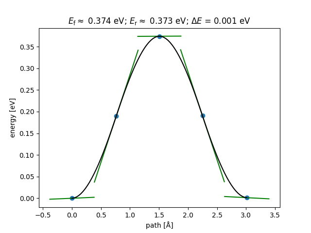
For more customizable analysis of the output of many NEB jobs, you can use the ase.mep.NEBTools class. Some examples of its use are below; the final example was used to make the figure you see above.

import matplotlib.pyplot as plt

from ase.io import read
from ase.mep import NEBTools

images = read('neb.traj@-5:')

nebtools = NEBTools(images)

Get the calculated barrier and the energy change of the reaction.

Ef, dE = nebtools.get_barrier()

Get the barrier without any interpolation between highest images.

Ef, dE = nebtools.get_barrier(fit=False)

Get the actual maximum force at this point in the simulation.

max_force = nebtools.get_fmax()

/home/ase/.local/lib/python3.13/site-packages/ase/mep/neb.py:329: UserWarning: The default method has changed from 'aseneb' to 'improvedtangent'. The 'aseneb' method is an unpublished, custom implementation that is not recommended as it frequently results in very poor bands. Please explicitly set method='improvedtangent' to silence this warning, or set method='aseneb' if you strictly require the old behavior (results may vary). See: https://gitlab.com/ase/ase/-/merge_requests/3952
  warnings.warn(

Create a figure like that coming from ASE-GUI.

fig = nebtools.plot_band()

$$E_\mathrm{f} \approx$ 0.374 eV; $E_\mathrm{r} \approx$ 0.373 eV; $\Delta E$ = 0.001 eV$

Create a figure with custom parameters.

fig = plt.figure(figsize=(5.5, 4.0))
ax = fig.add_axes((0.15, 0.15, 0.8, 0.75))
nebtools.plot_band(ax)

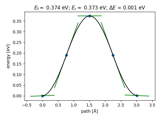
$$E_\mathrm{f} \approx$ 0.374 eV; $E_\mathrm{r} \approx$ 0.373 eV; $\Delta E$ = 0.001 eV$

<Figure size 550x400 with 1 Axes>

Note

For this reaction, the reaction coordinate is very simple: The x-coordinate of the Au atom. In such cases, the NEB method is overkill, and a simple constraint method should be used like in this tutorial: Surface diffusion energy barriers using ASE constraints.

Restarting NEB#

Restart NEB from the trajectory file:

read the last structures (of 5 images used in NEB)

images = read('neb.traj@-5:')

for i in range(1, len(images) - 1):
    images[i].calc = EMT()

neb = NEB(images, method='improvedtangent')
qn = BFGS(neb, trajectory='neb_restart.traj')
qn.run(fmax=0.005)

      Step     Time          Energy          fmax
BFGS:    0 15:12:53        3.688737        0.028898
BFGS:    1 15:12:53        3.688734        0.026547
BFGS:    2 15:12:53        3.688731        0.021515
BFGS:    3 15:12:53        3.688730        0.021379
BFGS:    4 15:12:53        3.688718        0.009577
BFGS:    5 15:12:53        3.688718        0.008389
BFGS:    6 15:12:53        3.688718        0.009122
BFGS:    7 15:12:53        3.688718        0.009290
BFGS:    8 15:12:53        3.688716        0.007568
BFGS:    9 15:12:53        3.688714        0.005563
BFGS:   10 15:12:53        3.688715        0.002547

np.True_

Parallelizing over images with MPI#

Instead of having one process do the calculations for all three internal images in turn, it will be faster to have three processes do one image each. In order to be able to run python with MPI you need a special parallel python interpreter, for example gpaw python (see GPAW parallel runs) and set parallel=True in the NEB calculation.

The example below can then be run with gpaw -P3 python diffusion_parallel.py:

initial = read('initial.traj')
final = read('final.traj')

constraint = FixAtoms(mask=[atom.tag > 1 for atom in initial])

n_images = 1  # Set to number of processes you use with mpiexec
images = [initial]
j = world.rank * n_images // world.size  # my image number
for i in range(n_images):
    image = initial.copy()
    if i == j:
        image.calc = EMT()
    image.set_constraint(constraint)
    images.append(image)
images.append(final)

neb = NEB(images, parallel=True, method='improvedtangent')
neb.interpolate()
qn = BFGS(neb, trajectory='neb.traj')
qn.run(fmax=0.05)

      Step     Time          Energy          fmax
BFGS:    0 15:12:53        4.219952        3.520752
BFGS:    1 15:12:53        3.937039        2.176459
BFGS:    2 15:12:53        3.730687        0.621235
BFGS:    3 15:12:53        3.710767        0.211379
BFGS:    4 15:12:53        3.707518        0.163942
BFGS:    5 15:12:53        3.704890        0.187028
BFGS:    6 15:12:53        3.699676        0.197511
BFGS:    7 15:12:53        3.694802        0.156084
BFGS:    8 15:12:53        3.691892        0.081850
BFGS:    9 15:12:53        3.691165        0.050493
BFGS:   10 15:12:53        3.690969        0.048196

np.True_

Gallery generated by Sphinx-Gallery

Surface diffusion energy barriers using the Nudged Elastic Band (NEB) method

Contents

Surface diffusion energy barriers using the Nudged Elastic Band (NEB) method#

Restarting NEB#

Parallelizing over images with MPI#