
Note
Go to the end to download the full example code.
NEB and Dimer method for Self-diffusion on the Al(110) surface#
In this exercise, we will find minimum-energy paths and transition states
using the Nudged Elastic Band method. We will illustrate
how NEB can be used in ASE to compute and compare three different
diffusion pathways for an Al atom
on a Al(110) surface. Finally, another method
for finding the transition state (i.e. the highest-energy state), the Dimer
method, will also be explored.
Initialize the system#
Al(110) surface can be generated with ASE code
Create Atoms object and
Multiply the unit cell to make it larger in x,y,z
initial *= (4, 4, 2)
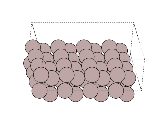
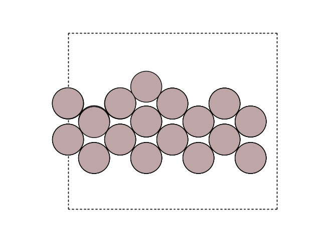
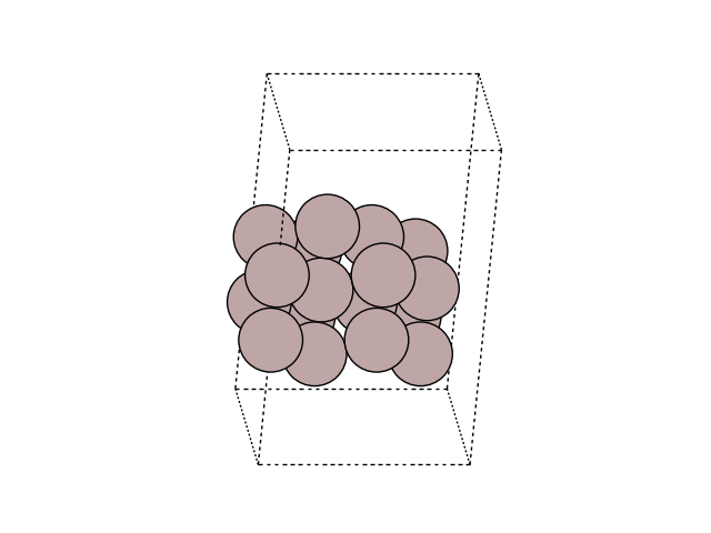
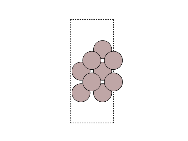
You can visualize the surface using
import matplotlib.pyplot as plt
from ase.visualize.plot import plot_atoms
fig, ax = plt.subplots()
plot_atoms(initial, ax, rotation=('-60x, 10y,0z'))
ax.set_axis_off()
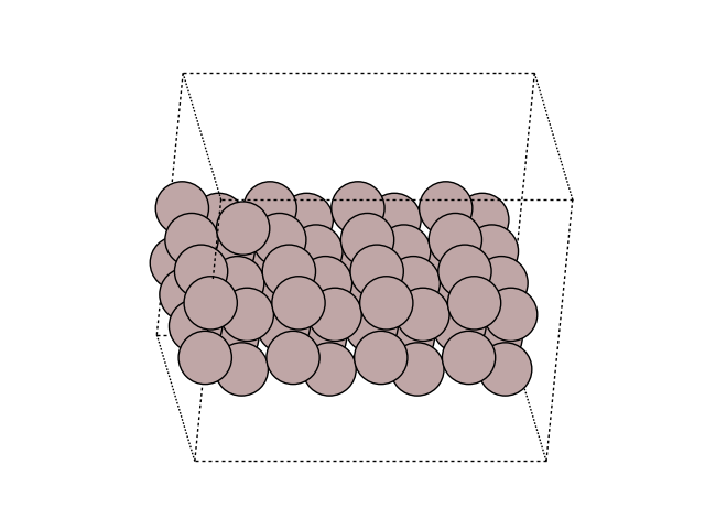
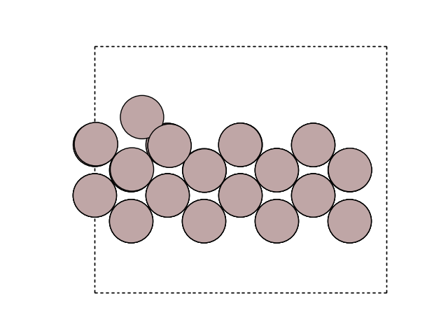
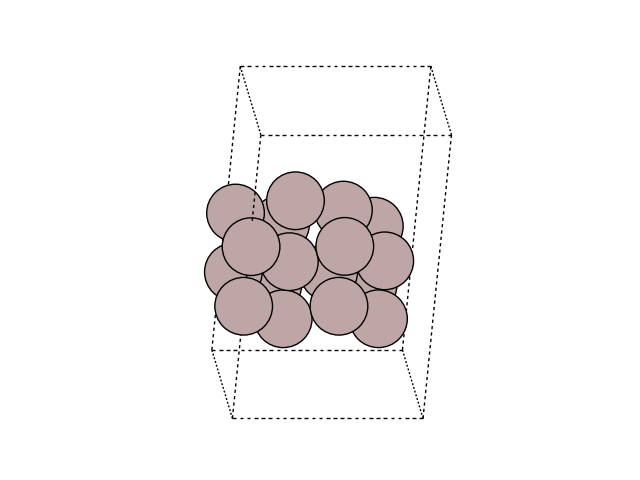
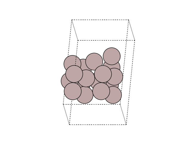
Then, lets add the Al addatom which will be the one moving on the surface.
Center the cell in vacuum along the z axis
initial.center(vacuum=4.0, axis=2)
Visualize the new atom in the cell
fig, ax = plt.subplots()
plot_atoms(initial, ax, rotation=('-60x, 10y,0z'))
ax.set_axis_off()

Perform a NEB calculation#
The adatom can jump along the rows (into the picture) or across
the rows (to the right inthe picture).
We are going to compute this motion to find out which of the two jump
will have the largest energy barrier.
To do this, you need to create an image with the atoms at
their final position.
First copy the initial Atoms object
final = initial.copy()
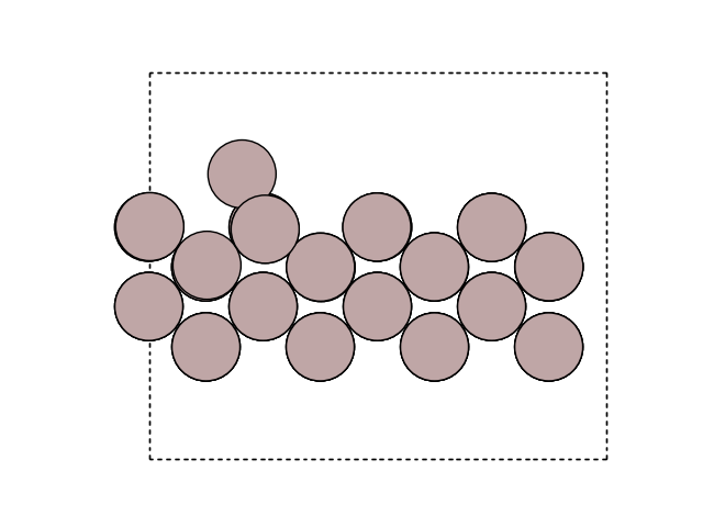
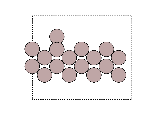
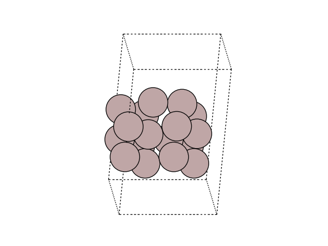
Then move the last atom of the Atoms object “final”
(the one atom we just added before) of +b along the second positional array
final.positions[-1, 1] += b
Visualize the new atom in the cell
fig, ax = plt.subplots()
plot_atoms(final, ax, rotation=('-60x, 10y,0z'))
ax.set_axis_off()
Let us fix the atoms that are not moving by creating a constraint and setting this constraint to the images. To do this, we create a mask of boolean array that select fixed atoms (the two bottom layers):
from ase.calculators.emt import EMT
from ase.constraints import FixAtoms
mask = initial.positions[:, 2] - min(initial.positions[:, 2]) < 1.5 * h
constraint = FixAtoms(mask=mask)
print(mask)
[ True True False False True True False False True True False False
True True False False True True False False True True False False
True True False False True True False False True True False False
True True False False True True False False True True False False
True True False False True True False False True True False False
True True False False False]
Set the FixAtoms to the Atoms objects,
and in the same loop, set the calculator (in this example we use EMT,
but you can use any calculator supported by ASE)
initial.calc = EMT()
initial.set_constraint(constraint)
final.calc = EMT()
final.set_constraint(constraint)
Use emt calculator and
QuasiNewton Algorithm to optimize
the geometry of the initial and final states
from ase.optimize import QuasiNewton
QuasiNewton(initial).run(fmax=0.05)
QuasiNewton(final).run(fmax=0.05)
Step[ FC] Time Energy fmax
BFGSLineSearch: 0[ 0] 18:46:10 17.939914 0.2540
BFGSLineSearch: 1[ 2] 18:46:10 17.897422 0.1631
BFGSLineSearch: 2[ 4] 18:46:10 17.884347 0.0522
BFGSLineSearch: 3[ 5] 18:46:10 17.881710 0.0269
Step[ FC] Time Energy fmax
BFGSLineSearch: 0[ 0] 18:46:10 17.939914 0.2540
BFGSLineSearch: 1[ 2] 18:46:10 17.897422 0.1631
BFGSLineSearch: 2[ 4] 18:46:10 17.884347 0.0522
BFGSLineSearch: 3[ 5] 18:46:10 17.881710 0.0269
np.True_
Then, construct a list of images by copying the first image several time in an array and append to this list the final image
Because the .copy() method does not copy the calculator, you need to set a new one for the created images
for image in images:
image.calc = EMT()
image.set_constraint(constraint)
Create a Nudged Elastic Band (mep import NEB) object
/home/ase/.local/lib/python3.13/site-packages/ase/mep/neb.py:329: UserWarning: The default method has changed from 'aseneb' to 'improvedtangent'. The 'aseneb' method is an unpublished, custom implementation that is not recommended as it frequently results in very poor bands. Please explicitly set method='improvedtangent' to silence this warning, or set method='aseneb' if you strictly require the old behavior (results may vary). See: https://gitlab.com/ase/ase/-/merge_requests/3952
warnings.warn(
Make a starting guess for the minimum energy path by performing a linear interpolation from the initial to the final image
neb.interpolate()
Perform the NEB calculation minimizing the force below 0.05 eV/A
Step Time Energy fmax
MDMin: 0 18:46:10 18.237088 0.993544
MDMin: 1 18:46:10 18.190945 0.836011
MDMin: 2 18:46:10 18.105033 0.460778
MDMin: 3 18:46:10 18.056201 0.122138
MDMin: 4 18:46:10 18.035931 0.102285
MDMin: 5 18:46:10 18.022022 0.118145
MDMin: 6 18:46:10 18.010798 0.088852
MDMin: 7 18:46:10 18.005186 0.127228
MDMin: 8 18:46:10 18.003865 0.114049
MDMin: 9 18:46:10 18.001954 0.088821
MDMin: 10 18:46:10 18.000262 0.063304
MDMin: 11 18:46:10 17.998668 0.053980
MDMin: 12 18:46:10 17.997130 0.040716
np.True_
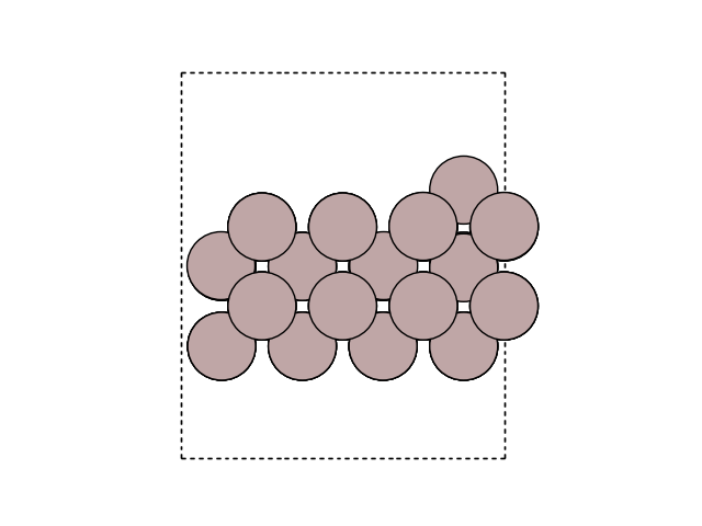
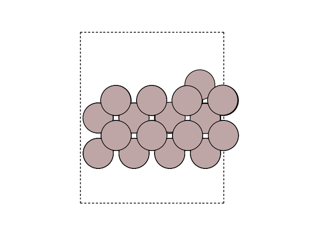
Visualize the minimum energy path (MEP) in side view to see the motion. Here, we look at the surface slab in yz direction.
for image in images:
fig, ax = plt.subplots()
plot_atoms(image, ax, rotation=('-90x, 90y,0z'))
ax.set_axis_off()


Plot the variation of potential energy
potential_energies = [image.get_potential_energy() for image in images]
fig, ax = plt.subplots()
plt.plot(
range(len(potential_energies)),
potential_energies - potential_energies[0],
marker='+',
)
plt.xlabel('Image number')
plt.ylabel('Potential energy (eV)')
diff = np.max(potential_energies) - potential_energies[0]
print(f'The energy barrier is {diff:.4f} eV.')
The energy barrier is 0.1154 eV.
You can visualize the NEB path using ASE GUI after saving the tajectory in a file
Otherwise, you can use ase gui neb_path.traj command in your terminal and
visualize the energy curve by plotting i, E[i] - E[1].
You now can answer those questions :
How is the shape of the potential (symmetric/asymmetric) and does this make sense for this process (when looking at the moving adatom in the simulation)?
What is the energy barrier?
Beyond your first NEB calculation#
You now can redo the same process to find the energy barrier to cross one row. The following code will produce the result (by making use of the previously initialized code), though we encourage you to try by yourself.
final = initial.copy()
final.positions[-1, 0] += a
Plot the images
for image in [initial, final]:
fig, ax = plt.subplots()
plot_atoms(image, ax, rotation=('-90x, 0y, 0z'))
ax.set_axis_off()

Construct a list of images:
Make a mask of zeros and ones that select fixed atoms (the two bottom layers):
mask = initial.positions[:, 2] - min(initial.positions[:, 2]) < 1.5 * h
constraint = FixAtoms(mask=mask)
print(mask)
for image in images:
# Let all images use an EMT calculator:
image.calc = EMT()
image.set_constraint(constraint)
[ True True False False True True False False True True False False
True True False False True True False False True True False False
True True False False True True False False True True False False
True True False False True True False False True True False False
True True False False True True False False True True False False
True True False False False]
Relax the initial and final states:
QuasiNewton(initial).run(fmax=0.05)
QuasiNewton(final).run(fmax=0.05)
Step[ FC] Time Energy fmax
BFGSLineSearch: 0[ 0] 18:46:13 17.881710 0.0269
Step[ FC] Time Energy fmax
BFGSLineSearch: 0[ 0] 18:46:13 17.898108 0.2165
BFGSLineSearch: 1[ 2] 18:46:13 17.883509 0.0755
BFGSLineSearch: 2[ 4] 18:46:13 17.880775 0.0216
np.True_
Create a Nudged Elastic Band:
Make a starting guess for the minimum energy path (a straight line from the initial to the final state):
neb.interpolate()
Relax the NEB path:
Step Time Energy fmax
MDMin: 0 18:46:13 21.182521 7.493573
MDMin: 1 18:46:13 19.417286 3.689216
MDMin: 2 18:46:13 18.645079 0.922870
MDMin: 3 18:46:13 18.533896 0.503897
MDMin: 4 18:46:13 18.525368 0.439764
MDMin: 5 18:46:13 18.507383 0.263744
MDMin: 6 18:46:13 18.491239 0.227551
MDMin: 7 18:46:13 18.479659 0.160835
MDMin: 8 18:46:13 18.468241 0.152303
MDMin: 9 18:46:13 18.458050 0.091391
MDMin: 10 18:46:13 18.450556 0.112507
MDMin: 11 18:46:14 18.447753 0.095248
MDMin: 12 18:46:14 18.447405 0.085207
MDMin: 13 18:46:14 18.446629 0.058262
MDMin: 14 18:46:14 18.445840 0.046679
np.True_
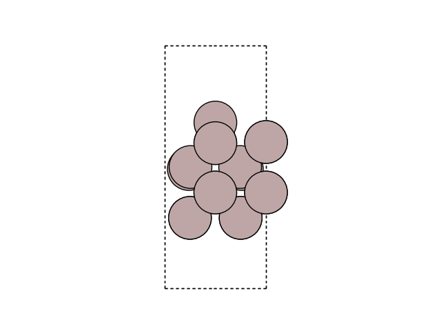
Visualize the MEP in side view to see the motion. We are now viewing the xz direction of the cell.
for image in images:
fig, ax = plt.subplots()
plot_atoms(image, ax, rotation=('-90x, 0y, 0z'))
ax.set_axis_off()

Plot the variation of potential energy
potential_energies = [image.get_potential_energy() for image in images]
fig, ax = plt.subplots()
plt.plot(
range(len(potential_energies)),
potential_energies - potential_energies[0],
marker='+',
)
plt.xlabel('Image number')
plt.ylabel('Potential energy (eV)')
diff = np.max(potential_energies) - potential_energies[0]
print(f'The energy barrier is {diff:.4f} eV.')
The energy barrier is 0.5641 eV.
Finding the third mechanism#
A third diffusion process can be found: Diffusion by an exchange process.
You can read more about it in the paper listed here.
Find the barrier for this process, and compare the energy barrier
with the two other ones.
The following code will produce the result (by making use of the previously
initialized code), though we encourage you to try by yourself.
a = 4.0614
b = a / sqrt(2)
h = b / 2
initial = Atoms(
    'Al2',
    positions=[(0, 0, 0), (a / 2, b / 2, -h)],
    cell=(a, b, 2 * h),
    pbc=(1, 1, 0),
)
initial *= (2, 2, 2)
initial.append(Atom('Al', (a / 2, b / 2, 3 * h)))
initial.center(vacuum=4.0, axis=2)
final = initial.copy()
# move adatom to row atom 14
final.positions[-1, :] = initial.positions[14]
# Move row atom 14 to the next row
final.positions[14, :] = initial.positions[-1] + [a, b, 0]
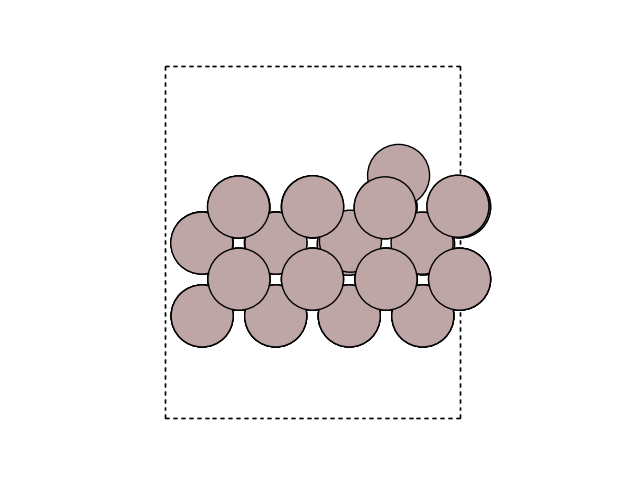
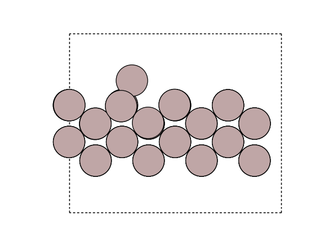
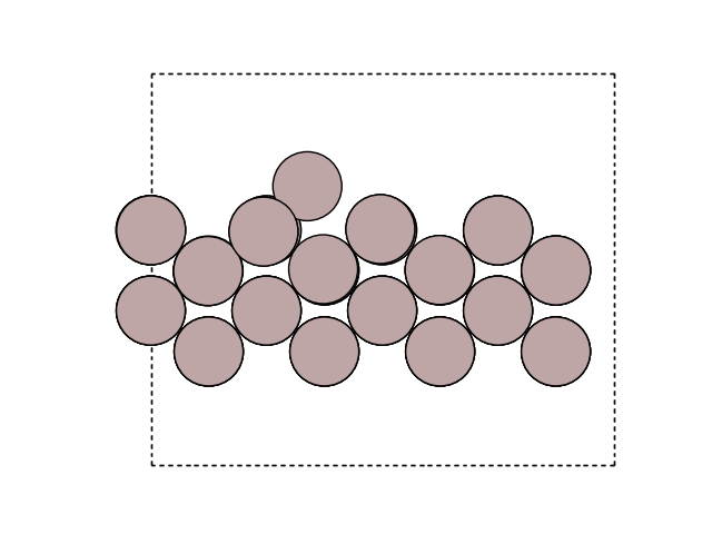
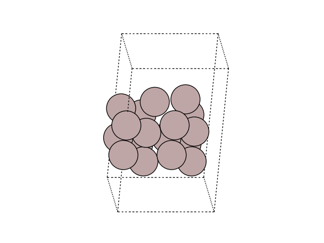
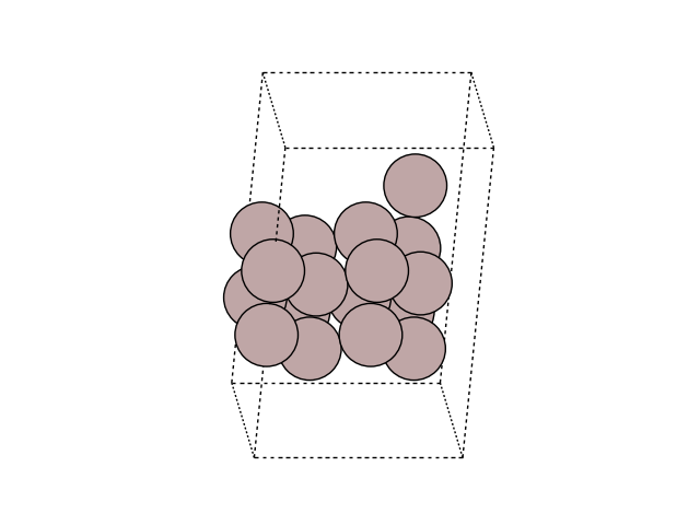
Visualize the initial and final images
for image in [initial, final]:
fig, ax = plt.subplots()
plot_atoms(image, ax, rotation=('-60x, 10y,0z'))
ax.set_axis_off()


Construct a list of images:
Make a mask of zeros and ones that select fixed atoms (the two bottom layers):
mask = initial.positions[:, 2] - min(initial.positions[:, 2]) < 1.5 * h
constraint = FixAtoms(mask=mask)
print(mask)
[ True True False False True True False False True True False False
True True False False False]
Let all images use an EMT calculator:
for image in images:
    image.calc = EMT()
    image.set_constraint(constraint)
Relax the initial and final states:
QuasiNewton(initial).run(fmax=0.05)
QuasiNewton(final).run(fmax=0.05)
Step[ FC] Time Energy fmax
BFGSLineSearch: 0[ 0] 18:46:16 4.639215 0.2538
BFGSLineSearch: 1[ 2] 18:46:16 4.622063 0.1580
BFGSLineSearch: 2[ 4] 18:46:16 4.613340 0.0622
BFGSLineSearch: 3[ 5] 18:46:16 4.611640 0.0336
Step[ FC] Time Energy fmax
BFGSLineSearch: 0[ 0] 18:46:16 4.639215 0.2538
BFGSLineSearch: 1[ 2] 18:46:16 4.622063 0.1580
BFGSLineSearch: 2[ 4] 18:46:16 4.613340 0.0622
BFGSLineSearch: 3[ 5] 18:46:16 4.611640 0.0336
np.True_
Create a Nudged Elastic Band:
Make a starting guess for the minimum energy path (a straight line from the initial to the final state):
neb.interpolate()
Relax the NEB path:
Step Time Energy fmax
MDMin: 0 18:46:16 5.433815 1.152831
MDMin: 1 18:46:16 5.352153 1.037842
MDMin: 2 18:46:16 5.179224 0.774873
MDMin: 3 18:46:16 5.033743 0.467209
MDMin: 4 18:46:16 4.952171 0.268936
MDMin: 5 18:46:16 4.905037 0.159289
MDMin: 6 18:46:16 4.877853 0.127328
MDMin: 7 18:46:16 4.868893 0.137692
MDMin: 8 18:46:16 4.868167 0.128909
MDMin: 9 18:46:17 4.866425 0.108529
MDMin: 10 18:46:17 4.864372 0.092540
MDMin: 11 18:46:17 4.862194 0.087441
MDMin: 12 18:46:17 4.859889 0.083497
MDMin: 13 18:46:17 4.857550 0.078463
MDMin: 14 18:46:17 4.855276 0.071014
MDMin: 15 18:46:17 4.853106 0.058560
MDMin: 16 18:46:17 4.851041 0.045468
np.True_
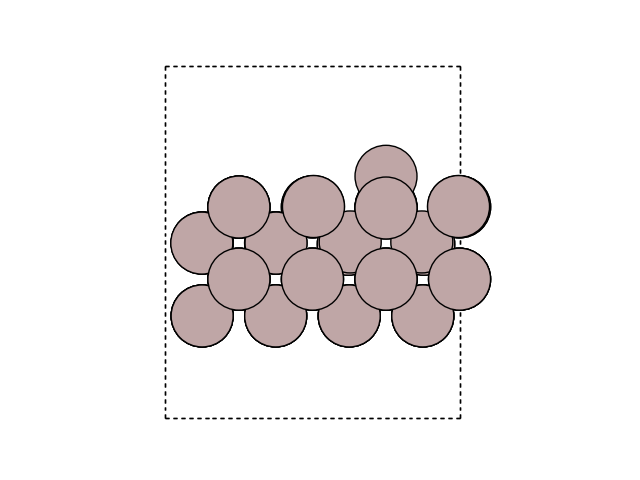
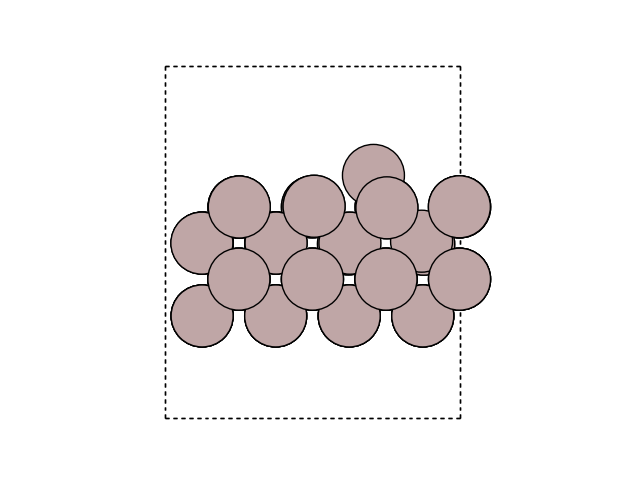
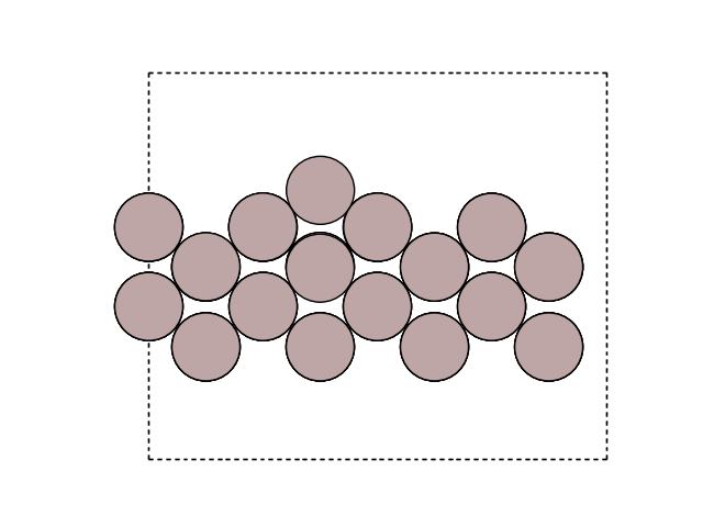
Visualize the MEP in side view to see the motion
for image in images:
fig, ax = plt.subplots()
plot_atoms(image, ax, rotation=('-60x, 10y,0z'))
ax.set_axis_off()

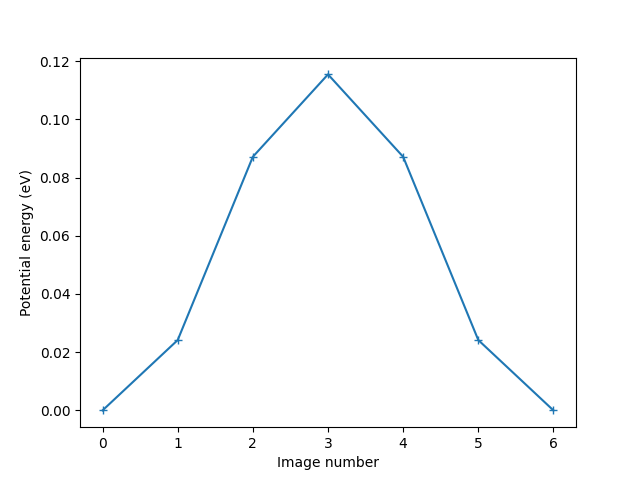
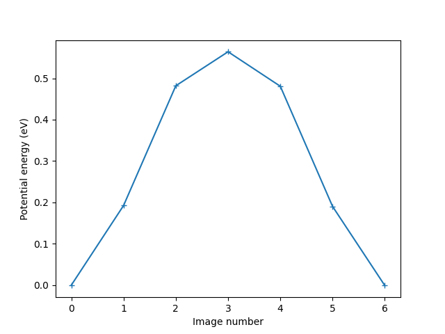
Plot the variation of potential energy
potential_energies = [image.get_potential_energy() for image in images]

fig, ax = plt.subplots()
plt.plot(
    range(len(potential_energies)),
    potential_energies - potential_energies[0],
    marker='+',
)
plt.xlabel('Image number')
plt.ylabel('Potential energy (eV)')

diff = np.max(potential_energies) - potential_energies[0]
print(f'The energy barrier is {diff:.4f} eV.')
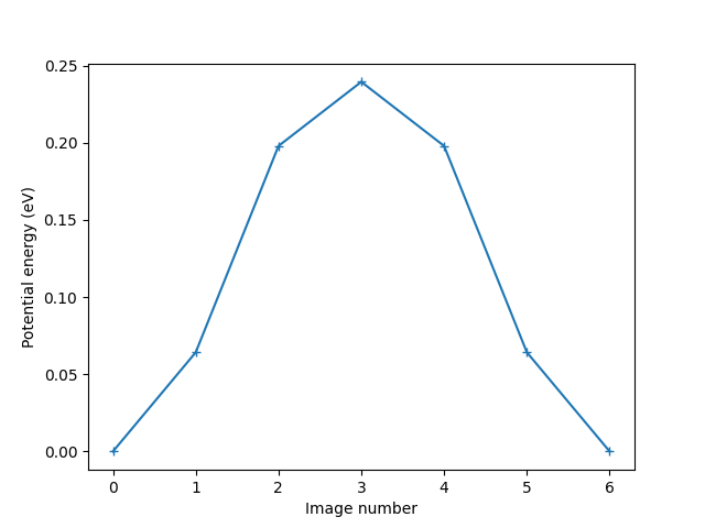
The energy barrier is 0.2394 eV.
Hint
When opening a trajectory with ase gui with calculated energies, the default plot window shows the energy versus frame number. To get a better feel of the energy barrier in an NEB calculation; choose . This will give a smooth curve of the energy as a function of the NEB path length, with the slope at each point estimated from the force.
Performing Dimer-method calculation#
In the NEB calculations above we knew the final states, so all we had
to do was to calculate the path between the initial state
and the final state.
But in some cases we do not know the final state.
Then the Dimer method can be used to
find the transition state.
The result of a Dimer calculation will hence not be the complete particle
trajectory as in the NEB output, but rather the configuration of
the transition-state image.
The following code will find the transition-state image of the jump along the row.
from ase.io import Trajectory
from ase.mep import DimerControl, MinModeAtoms, MinModeTranslate

a = 4.0614
b = a / sqrt(2)
h = b / 2
initial = Atoms(
    'Al2',
    positions=[(0, 0, 0), (a / 2, b / 2, -h)],
    cell=(a, b, 2 * h),
    pbc=(1, 1, 0),
)
initial *= (2, 2, 2)
initial.append(Atom('Al', (a / 2, b / 2, 3 * h)))
initial.center(vacuum=4.0, axis=2)


initial_copy = initial.copy()

N = len(initial)  # number of atoms


# Make a mask of zeros and ones that select fixed atoms - the two
# bottom layers:
mask = initial.positions[:, 2] - min(initial.positions[:, 2]) < 1.5 * h
constraint = FixAtoms(mask=mask)
initial.set_constraint(constraint)

# Calculate using EMT:
initial.calc = EMT()

# Relax the initial state:
QuasiNewton(initial).run(fmax=0.05)
e0 = initial.get_potential_energy()

# To save the trajectory file
traj = Trajectory('dimer_along.traj', 'w', initial)
traj.write()
                Step[ FC]     Time          Energy          fmax
BFGSLineSearch:    0[  0] 18:46:18        4.639215       0.2538
BFGSLineSearch:    1[  2] 18:46:18        4.622063       0.1580
BFGSLineSearch:    2[  4] 18:46:18        4.613340       0.0622
BFGSLineSearch:    3[  5] 18:46:18        4.611640       0.0336
Making dimer mask list:
d_mask = [False] * (N - 1) + [True]

# Set up the dimer:
d_control = DimerControl(
    initial_eigenmode_method='displacement',
    displacement_method='vector',
    logfile=None,
    mask=d_mask,
)
d_atoms = MinModeAtoms(initial, d_control)

# Displacement settings:
displacement_vector = np.zeros((N, 3))
# Strength of displacement along y axis = along row:
displacement_vector[-1, 1] = 0.001
# The direction of the displacement is set by the a in
# displacement_vector[-1, a], where a can be 0 for x, 1 for y and 2 for z.
d_atoms.displace(displacement_vector=displacement_vector)

# Converge to a saddle point:
dim_rlx = MinModeTranslate(d_atoms, trajectory=traj, logfile=None)
dim_rlx.run(fmax=0.001)
np.True_
Visualize the Initial state and the saddle point in side view to see the change
for image in [initial, initial_copy]:
    fig, ax = plt.subplots()
    plot_atoms(image, ax, rotation=('-90x, 90y,0z'))
    ax.set_axis_off()


diff = initial.get_potential_energy() - e0
print(f'The energy barrier is {diff:.4f} eV.')
The energy barrier is 0.1090 eV.
Compare the transition-state images of the NEB and Dimer as viewed in the GUI. Are they identical?
What is the energy barrier? How does it compare to the one found in the NEB calculation?
Do the same as above for the jump across the row and the exchange process by copying and modifying the Dimer script, while remembering that you have to give the relevant atoms a kick in a meaningful direction.