Constrained Calculations - Surface diffusion energy barriers#

In this tutorial, we will calculate the energy barrier that was found using the NEB method in the Surface diffusion energy barriers using the Nudged Elastic Band (NEB) method tutorial. Here, we use a simple FixedPlane constraint that forces the Au atom to relax in the yz-plane only:

from ase.build import add_adsorbate, fcc100
from ase.calculators.emt import EMT
from ase.constraints import FixAtoms, FixedPlane
from ase.optimize import QuasiNewton

# 2x2-Al(001) surface with 3 layers and an
# Au atom adsorbed in a hollow site:
slab = fcc100('Al', size=(2, 2, 3))
add_adsorbate(slab, 'Au', 1.7, 'hollow')
slab.center(axis=2, vacuum=4.0)

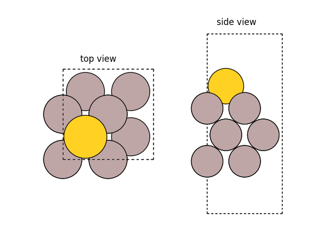
We can visualize the structure with ase visualize:

import matplotlib.pyplot as plt

from ase.visualize.plot import plot_atoms

fig, (ax1, ax2) = plt.subplots(1, 2)
plot_atoms(slab, ax1)
plot_atoms(slab, ax2, rotation='-90x')
ax1.set_title('top view')
ax2.set_title('side view')
ax1.set_axis_off()
ax2.set_axis_off()

Alternatively, you can use also use view directly:

#   $ from ase.visualize import view
#   $ view(slab)

We can now continue fixing the atoms in the slab:

# Fix second and third layers:
mask = [atom.tag > 1 for atom in slab]
# print(mask)
fixlayers = FixAtoms(mask=mask)

# Constrain the last atom (Au atom) to move only in the yz-plane:
plane = FixedPlane(-1, (1, 0, 0))

slab.set_constraint([fixlayers, plane])

Now we can perform the calculation optimizing the displacement of the gold atom along the x-axis. We do structure optimization here using the EMT potential:

# Use EMT potential:
slab.calc = EMT()

for i in range(5):
    qn = QuasiNewton(slab, trajectory=f'mep{i}.traj')
    qn.run(fmax=0.05)
    # Move gold atom along x-axis:
    slab[-1].x += slab.get_cell()[0, 0] / 8

# Let's visualize the saved trajectory.
# Here is code to visualize
# a side-view of the path (unit cell repeated twice):


from ase.io import read

configs = [read(f'mep{i}.traj', '-1') for i in range(5)]

# for easier visualization, let's repeat the structures
configs_repeated = [config.repeat((2, 1, 1)) for config in configs]

                Step[ FC]     Time          Energy          fmax
BFGSLineSearch:    0[  0] 10:57:13        3.323870       0.2462
BFGSLineSearch:    1[  1] 10:57:13        3.314754       0.0378
                Step[ FC]     Time          Energy          fmax
BFGSLineSearch:    0[  0] 10:57:13        3.730166       1.6460
BFGSLineSearch:    1[  2] 10:57:13        3.546230       0.2605
BFGSLineSearch:    2[  4] 10:57:13        3.513795       0.1080
BFGSLineSearch:    3[  6] 10:57:13        3.502279       0.0500
                Step[ FC]     Time          Energy          fmax
BFGSLineSearch:    0[  0] 10:57:13        3.764262       1.0444
BFGSLineSearch:    1[  2] 10:57:13        3.708446       0.1203
BFGSLineSearch:    2[  4] 10:57:13        3.695835       0.0668
BFGSLineSearch:    3[  6] 10:57:13        3.691660       0.0618
BFGSLineSearch:    4[  7] 10:57:13        3.690089       0.0300
                Step[ FC]     Time          Energy          fmax
BFGSLineSearch:    0[  0] 10:57:13        3.580034       0.6521
BFGSLineSearch:    1[  1] 10:57:13        3.544894       0.1627
BFGSLineSearch:    2[  3] 10:57:13        3.516850       0.1946
BFGSLineSearch:    3[  4] 10:57:13        3.508545       0.1325
BFGSLineSearch:    4[  5] 10:57:13        3.503316       0.1022
BFGSLineSearch:    5[  6] 10:57:13        3.500392       0.0550
BFGSLineSearch:    6[  8] 10:57:13        3.499584       0.0392
                Step[ FC]     Time          Energy          fmax
BFGSLineSearch:    0[  0] 10:57:13        3.463634       0.5332
BFGSLineSearch:    1[  2] 10:57:13        3.356702       0.4028
BFGSLineSearch:    2[  3] 10:57:13        3.333298       0.1536
BFGSLineSearch:    3[  4] 10:57:13        3.322604       0.1003
BFGSLineSearch:    4[  5] 10:57:13        3.318477       0.0658
BFGSLineSearch:    5[  6] 10:57:13        3.316534       0.0483

We can visualize the structures with \(ase.visualize.plot.animate\):

from ase.visualize.plot import animate

animate(
    configs_repeated,
    ax=None,
    interval=500,  # in ms; same default value as in FuncAnimation
    rotation=('-90x,0y,0z'),
)

<matplotlib.animation.FuncAnimation object at 0x7f7755ca3e00>

Let’s plot the energy and look at the barrier.

# get the potential energies of the structures
energies = [config.get_potential_energy() for config in configs]
# set last energy value to 0 for easier comparison
energies = [energy - energies[-1] for energy in energies]
plt.ylabel(r'$E(i) - E_{\mathrm{final}}$ (meV)')
plt.xlabel('Image number')
plt.plot(range(1, len(energies) + 1), energies)

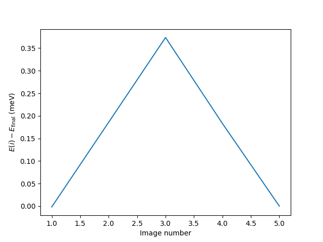
[<matplotlib.lines.Line2D object at 0x7f773bd04410>]

The barrier is found to be 0.35 eV - exactly as in the NEB tutorial.

The result can also be analysed with the command ase gui mep?.traj -n -1 (choose Tools ‣ NEB).